Ultrafast Laser Pulse Measurement
OBJECTIVES: The
accurate knowledge of the pulse width of the ultrafast laser pulse is of
paramount importance during any experiment in an ultrafast lab. While modern
day electronics can not measure any event faster than few Pico-seconds, there are
some other state of the art techniques available for characterizing the laser
pulses among which Autocorrelation is one of the most efficient techniques
which we practice regularly.
THEORY: As
the name suggests, the autocorrelation is the measurement of the pulse using
the original pulse itself. Experimentally the original pulse is split in two
equal parts and they are again made to recombine both specially and temporally
using a variable time delay in one arm. A detector placed at the recombination
point detects the interference between two pulses which in turn is converted to
the autocorrelation spectrum. Depending on the measurement process this can be
of two types- Intensity Autocorrelation and Field Autocorrelation.
Mathematically, autocorrelation
function is defined as
![]()
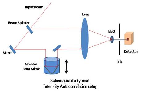
INTENSITY AUTOCORRELATION:
This is done using a
non-collinear geometry where the two arms are focused to a point using a lens
and a BBO is kept at the focal point. At this point the second harmonic
generated is proportional to ![]() which is the sum of three components. The
third component proportional to
which is the sum of three components. The
third component proportional to ![]() is our desired autocorrelation signal that is
detected by the detector as
is our desired autocorrelation signal that is
detected by the detector as
![]()
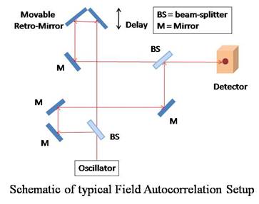
FIELD AUTOCORRELATION:
This is done in a collinear
geometry where two pulses are recombined collinearly and the signal detected by
the detector is given by
![]()
Where ![]() is the first order autocorrelation function. If we place
a BBO crystal in front of the detector and collect only the SHG signal we get
the interferrometric (second order) autocorrelation signal as before(look at
intensity autocorrelation for mathematical expression).
is the first order autocorrelation function. If we place
a BBO crystal in front of the detector and collect only the SHG signal we get
the interferrometric (second order) autocorrelation signal as before(look at
intensity autocorrelation for mathematical expression).
INSTRUMENTS UTILIZED:
1. LASER,
Mirrors, mirror holders.
2. Lenses,
lens holders, irises, retro mirror.
3. Beam
splitter,
4. Non Linear Crystal (BBO).
5.
Photo Diode.
6.
Oscilloscope, GPIB Card
7.
Motorized Linear Stage, Motorized Stage Controller
8.
BNC cable, GPIB connector.
9.
Laser glasses for eye safety.
SOFTWARE USED:
- LabVIEW software for data
acquisition.
- Origin pro for data plotting and analysis.
Note: For user operation and usage no specific
software needed.
EXPERIMENT PROCEDURE:
INTENSITY AUTOCORRELATION:
1.
Turn
ON the key Switch (from OFF to ON position).
2.
Wait
for 10-15 minutes.
3.
Open
the Shutter by pressing the shutter open switch and then press the power level
2 switch.
4.
Switch
on the Chiller.
5.
Wait
for 40-45 minutes for stabilization of the laser; put a power meter in the
optical path to measure the average power of the laser and then remove it.
6.
Make
the laser from CW to Mode Locked Condition.
7.
Put
one ultrafast thin Beam Splitter (BS), which divides the total optical path
into two parts. One path is call pump path and another is called probe path.
8.
Put
the Retro on a motorized stage in one path (Probe path) such that the beam
height at the input and at the output paths are same & the beam path
distances of the input and output paths are same up to 4-5 meter distances. If
the beam paths are not parallel then recheck the alignment.
9.
Align
the laser path according to schematic diagram (Fig: 1).
10. Measure the Optical
Path & make sure that the pump and probe path lengths are same, and make
the output beam paths parallel (both Pump and probe), If both are not parallel
then make it parallel and recheck the alignment properly.
11. Put one Plano convex
lens (15 mm) in to the parallel path such that Foci of the pump & probe
beams are same.
12. Put one thin BBO (SHG
crystal) in to the foci and rotate the BBO such that in the middle of the two
beam one extra signal is generated , which is SHG signal, if this signal is
absent then move the motorized stage such that the SHG signal is generated, if not recheck the alignment .
13. After SHG generation
keep a Photo Diode (PD) into the SHG path and collect the SHG signal through
digital Oscilloscope interfaced with GPIB to the computer.
14. Move the Motorized
stage and collect the SHG signal, after collecting data fit it into Gaussian
and measure the Full width at Half Maxima (FWHM) which is the pulse width of
the laser pulse.
FIELD AUTOCORRELATION:
1. Turn
ON the key Switch (from OFF to ON
position).
2. Wait
for 10-15 minutes.
3. Open
the Shutter by pressing the shutter open switch and then press the power level 2 switch.
4. Switch
on the Chiller.
5. Wait
for 40-45 minutes for stabilization of the laser; put a power meter in the
optical path to measure the average power of the laser and then remove it.
6. Make
the laser from CW to Mode Locked Condition.
7. Put
one ultrafast thin Beam Splitter (BS), which divides the total optical path
into two parts. One path is called pump path and another is called probe path.
8. Put
the Retro on a motorized stage in one path (Probe path) such that the beam
height at the input and at the output paths are same & the beam path
distances of the input and output paths are same up to 4-5 meter distances. If
the beam paths are not parallel then recheck the alignment.
9. Put
another ultrafast thin beam splitter in the crossing point of the pump and
probe beam such that they are fully overlapped in the transmitted and reflected
path, if they are not properly overlapped then recheck the alignment properly.
10. Align
the laser path according to schematic diagram (Fig: 3).
11. Measure
the Optical Path & make sure that the pump and probe path lengths are same.
When both the arm are of same lengths then we can see the fringes by putting a
white paper after the second beam splitter, if fringes are not visible, recheck
the alignment properly.
12. Put
one Plano convex lens (15 mm) in to the transmitted path.
13. After
checking the fringes pattern keep a Photo Diode (PD) into the optical path and
collect the signal through digital Oscilloscope interfaced with GPIB to the
computer.
14. Move
the Motorized stage and collect the signal, after collecting data fit it into
Gaussian and measure the Full width at Half Maxima (FWHM) which is the pulse
width of the laser pulse.