SST (Shear Stress Transport) Turbulence Model

A major concern in flow simulation is the separation from a surface under adverse pressure gradient. Separation has a strong effect on the near-wall turbulence and therefore on the turbulent heat transfer. The SST model, has demonstrated the capability of accurate separation predictions in numerous cases, and it is used as the basis for heat transfer predictions by many authors. The idea behind the SST model is to combine the best elements of the k - ε and the k - ω model with the help of a blending function F1. F1 is one near the surface and zero in the outer part and for free shear flows. It activates the Wilcox model (k-ω)in the near-wall region and the k - ε model for the rest of the flow. By this approach, the attractive near-wall performance of the Wilcox model can be utilized without the potential errors resulting from the free stream sensitivity of that model.

The formation of the SST model is as follows:

(28.5)

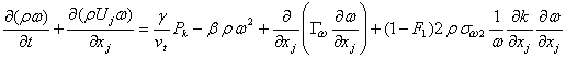(28.6)

with

(28.7)

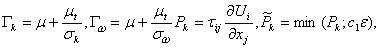
The coefficients, φ , of the model are functions F₁ : φ = F₁φ₁ + (1 - F₁ )φ₂ , where φ₁ , φ₂ stand for the coefficients of the k- ω and the k- ε model respectively:

σ k1 = 2.0, σω1 = 2.0, = 0.41, γ1 = 0.5532, β1 = 0.0750, β* = 0.09, c1 = 10

σ k2 = 1.0, σω2 = 1.168, = 0.41, γ2 = 0.4403, β2 = 0.0828, β* = 0.09,

with

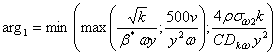	(28.8)
	(28.9)
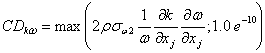
	(28.10)
	(28.11)

An additional feature of the SST model is the introduction of an upper limit for the turbulent shear stress in boundary layers in order to avoid excessive shear-stress levels typically predicted with Boussinesq eddy-viscosity models. The eddy viscosity is defined as:

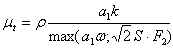(28.12)

With a₁ = 0.31. Again F2 is a blending function (described in Eq. (28.9)) similar to F1 , which restricts the limiter to the wall boundary layer, as the underlying assumptions are not correct for free shear flows.