Homework 2

Part A

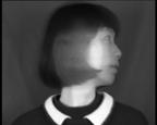
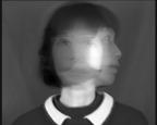
Original Image

m = 1

m = 2

m = 10

m = 30

m = 80

Part B

Plot of Residual Variance Vs Isomap Dimensionality

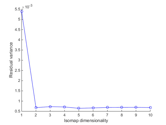
Table for Residual Variance of different dimensionality of Isomap

Isomap Dimensionality	1	2	3	4	5	6	7	8	9	10
Residual Variance	0.0053849,	0.00068328	0.0007271	0.00071342	0.00064705	0.00066579	0.00068959	0.00069323	0.00069579	0.00068443

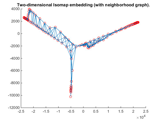
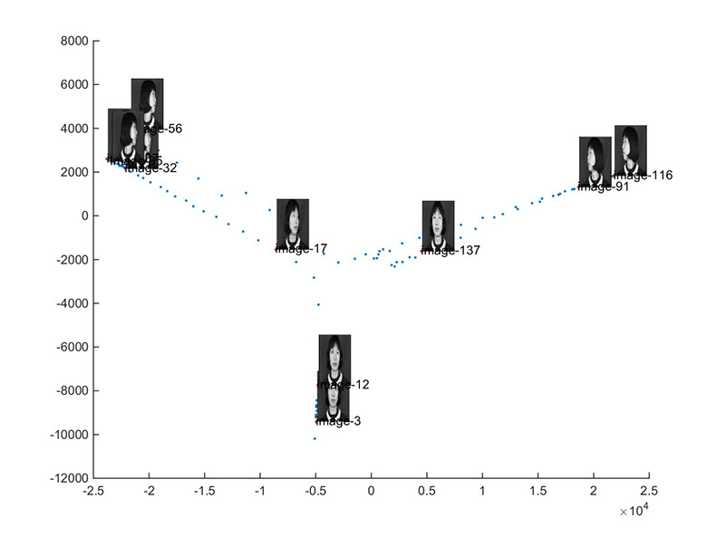
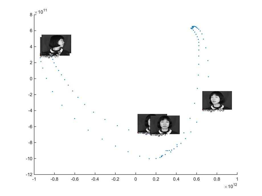
Plot of Two Dimensional Embedding of Isomap with some Random Images Shown

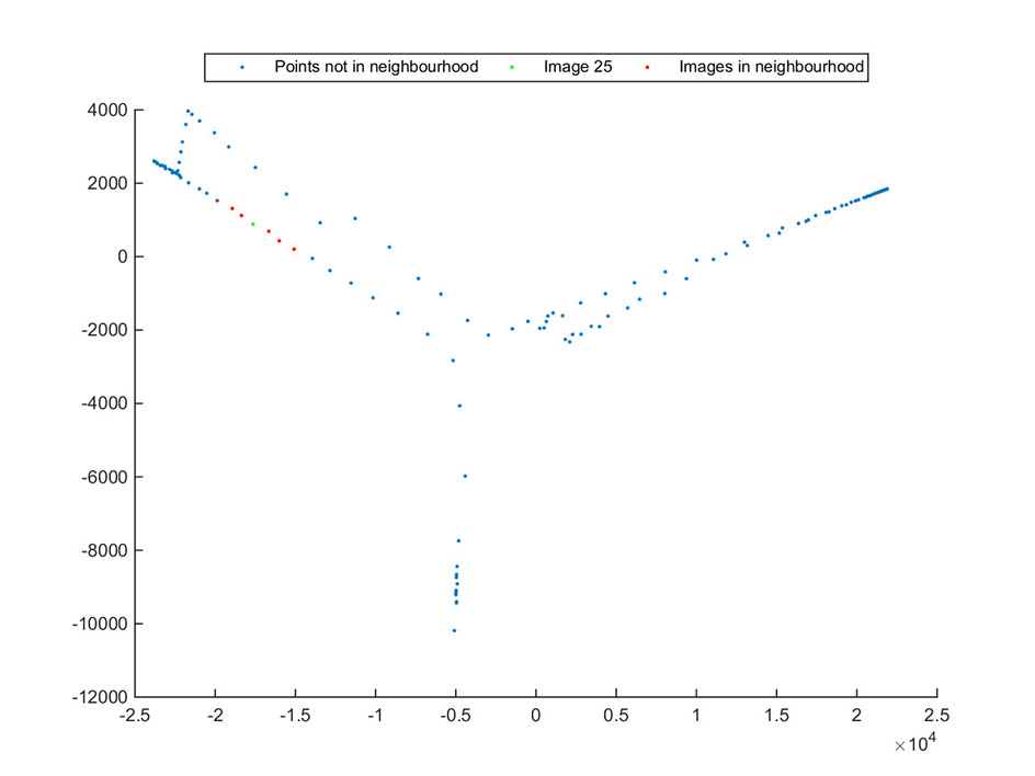
Plot of Neighborhood of Image 25 in 5-D Isomap Embedded in 2-D Isomap

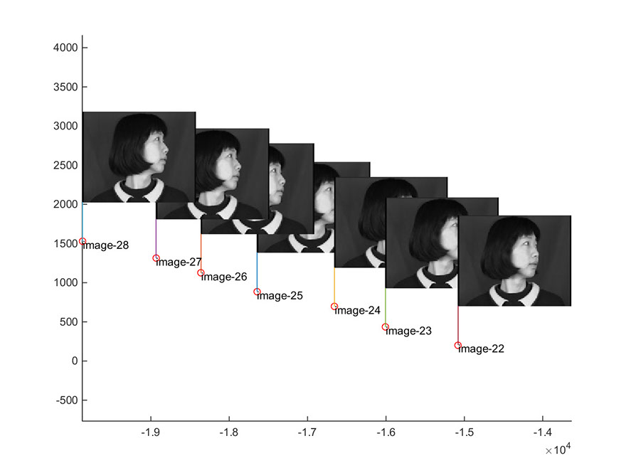
Zoomed-in image for Neighborhood of Image 25

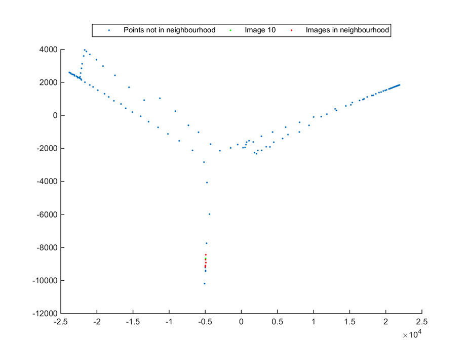
Plot of Neighborhood of Image 10 in 2-D Isomap

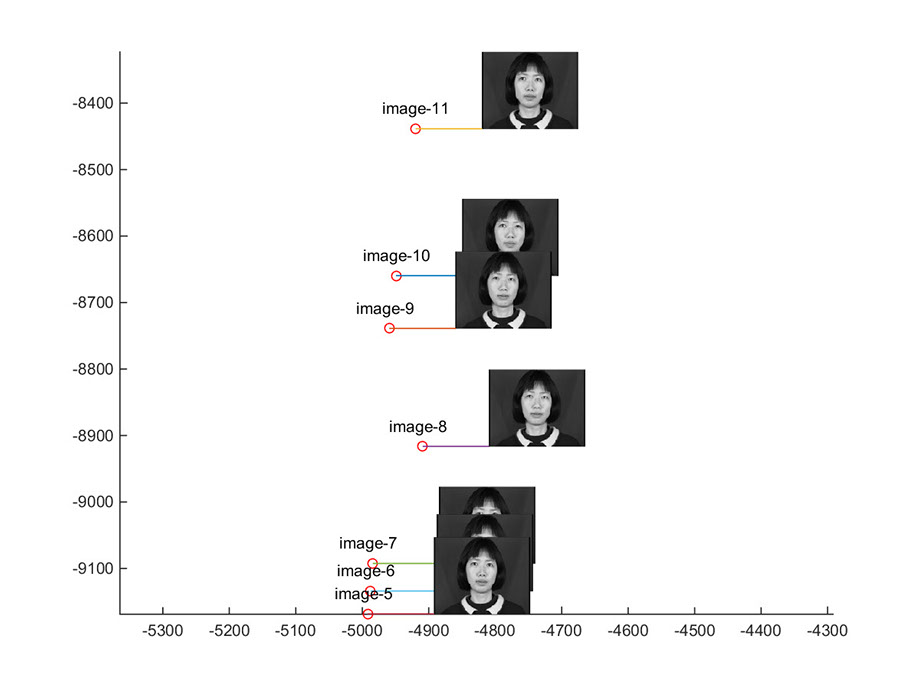
Zoomed-in image for Neighborhood of Image 10

Nature of the manifold in Isomap

The manifold in 2D can be described approximately as 3 lines intersecting each other. The lines correspond to the variations due to head turning right, then left and the center position. The manifold is expected to be a straight line in 2D because head is turning in one dimension only but due to other movements(like eye movement, tilt etc.) of the head while turning, the variations appear in the manifold.

Part C

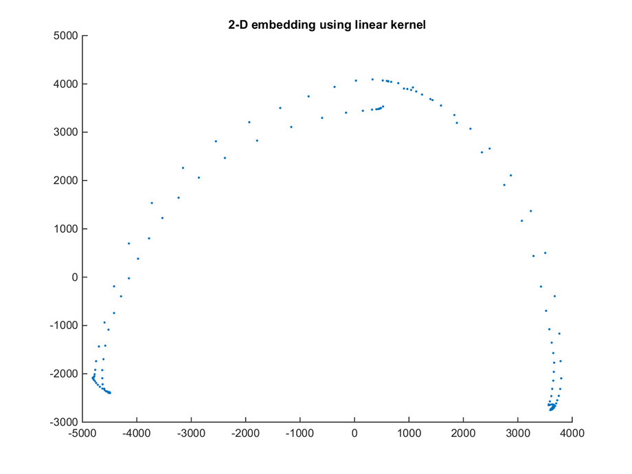
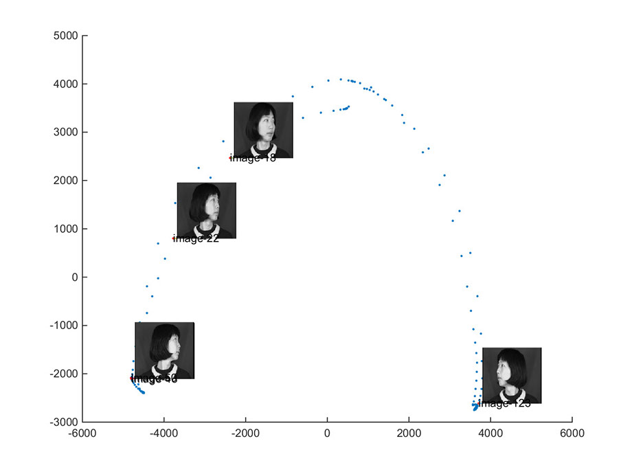
Randomly Selected Images shown in 2D Embedding using Linear Kernel

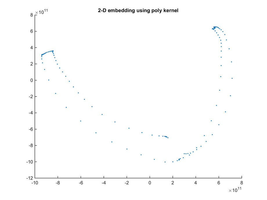
Randomly Selected Images shown in 2D Embedding using Poly Kernel

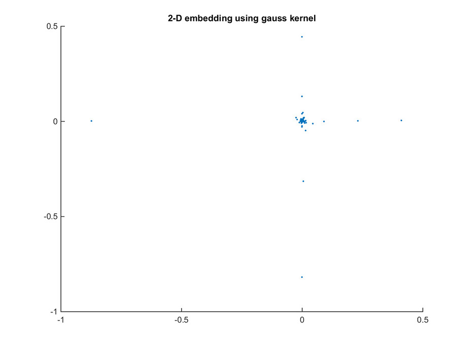
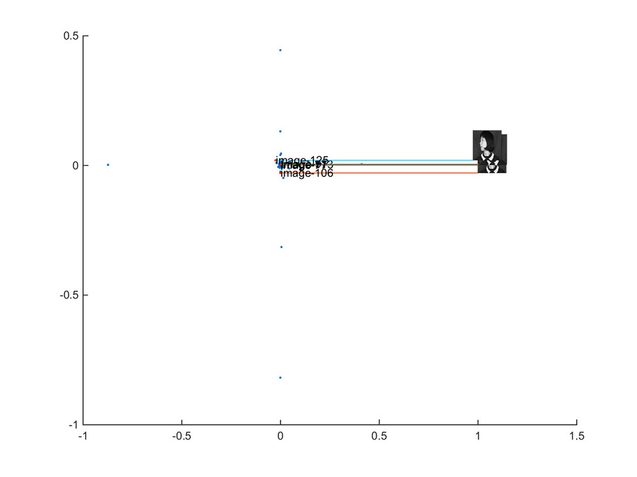
Randomly Selected Images shown in 2D Embedding using Gauss Kernel

Nature of the manifold in Kernel PCA

The 2D embedding for the given data is best described by poly and linear kernels. The data variation is mapped very poorly in case of gauss kernel.

Matlab Code used in this assignment can be found here.

Please refer to the README file for code usage and sources for Matlab Toolkits used.

m = 143