Engineering Hydrology by Rajesh Srivastava and Ashu Jain

McGraw Hill Education, New Delhi (2017)

TABLE OF CONTENTS

Errata: (Readers are encouraged to mail us either at rajeshs@iitk.ac.in or at ashujain@iitk.ac.in about any errors they spot)

Chapter-3: Abstractions

[1] Page 72: "(a) Penman method" should not have "(a)"

[2] Page 73: "(b) Actual Evaporation" should be "3.4.3 Actual Evaporation"

[3] Page 79: "3.5.2.2 Actual Evapotranspiration" should be "3.5.3 Actual Evapotranspiration"

Chapter-4: Runoff

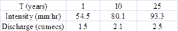
[1] Page 118: Example 4.2; Line 1: Area of catchment should be taken as 24 ha instead of 240 ha. As a result in the table on page 119, intensities should be 54.5, 80.1, and 93.3 and the peak discharges should be 1.5, 2.1, 2.5 for return periods of 1-year, 10-years, and 25-years, respectively. Thus, the modified table should look like this:

[2] Page 126: Example 4.3; Line 7: In expression V_R = P * A, "P" should be replaced by "ER".

Chapter-5: Hydrograph Analysis

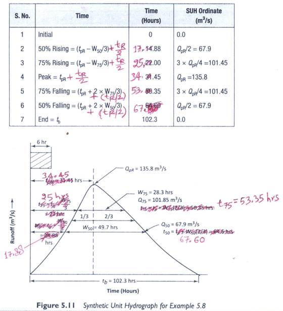
[1] On pages 166-167, Example 5.8: Please note that the time to peak calculated should be from the centroid of ERH and not the start of the ERH as shown. As such, t_R/2 (= 6/2 = 3 hours) needs to be added to the timings. The table and Figure 5.11 (on page 167) should therefore need to be modified as follows. Note that Q^s remain the same.

[2] Page 183, Q 5.2, last line: "Jun 30" should be read as "June 30".

Chapter-6: Hydrograph Routing

[1] On pages 193-194, Example 6.1: The entries in columns [5] to [8] are incorrect due to an inadvertent error in calculating elevation and outflow in the first row for t = 3 hours, which gets accumulated at later times. The modified table with correct entries in columns [5]-[8] is provided below with modified numbers in red-font.

Table of calculations for outflow hydrograph for EXAMPLE 6.1 on page 193-194

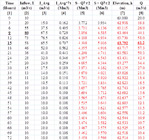
As a result, some of the numbers in the two paragraphs following this table (on page 194) get modified as follows (the modified numbers are represented in red font).

The computations for the routing of inflow hydrograph are carried out in a tabular form above. The first two columns of the table represent the given inflow hydrograph. Column 3 gives the average inflow value at each time interval, (I₁+I₂)/2 or (I_avg), in m³/s. Column 4 is the inflow volume in each time interval, (I_avgΔt), in Mm³, which is obtained by multiplying the entries in column 3 by 3 hours or 10,800 s. The first row against time t = 0 represents the initial conditions i.e. I = 10 m³/s, h = 63.000 m, and Q = 20 m³/s. For the given initial h = 63.000 m, we have S = 3.88 Mm³. Using the values of initial S and Q, we calculate (S-QΔt/2) = 3.772 Mm³. This is entered in column 5 in the row for t = 3 hours. Now as per equation (6.6), the RHS is calculated as the sum of column 4 and column 5. Therefore, (S+QΔt/2) = 3.934 Mm³, this is entered in column 6 in the row for t = 3. Now using the indicative storage graph prepared (Figure 6.1), we find out the values of elevation in the reservoir (h) and outflow (Q) corresponding to the value of (S+QΔt/2) = 3.934 Mm³ just calculated, by using the arrows. Note that this step can also be easily carried out by using linear interpolation of the (S+QΔt/2) v/s h and Q v/s h data. The values of h and Q are thus found as h = 62.965(62.938) m and Q = 24.9(18.8) m³/s, respectively; and are entered in column 7 and column 8, respectively, in the row for t = 3 hours. This completes the calculations for t = 3 hours. Now, using (S+QΔt/2) = 3.934 Mm³ at the end of 3 hours, we find (S-QΔt/2) = (S+QΔt/2) − QΔt = 3.665(3.731) Mm³. With the value of (S-QΔt/2) = 3.665(3.731) Mm³ at t = 6 hours, the RHS is calculated as the sum of column 4 and column 5, as per equation (6.6). Therefore, (S+QΔt/2) = 4.070(4.136) Mm³, this is entered in column 6 in the row for t = 6. Now using the indicative storage graph prepared (Figure 6.1), we find out the values of h and Q corresponding to the value of (S+QΔt/2) = 4.070(4.136) Mm³. The values of h and Q are thus found as h = 63.040(63.115) m and Q = 27.6(26.0) m³/s, respectively; and are entered in column 7 and column 8, respectively, in the row for t = 6 hours. This completes the calculations for t = 6 hours.

This process is then continued for each time step and the inflow hydrograph is thus routed through the reservoir to calculate the outflow hydrograph. The outflow hydrograph is presented in column 8 in the table above and the inflow and outflow hydrographs are shown in the figure below. Note that the peak flow of 80 m³/s occurs at t = 9 hours in the inflow hydrograph, while the peak flow of 59.9(61.2) m³/s occurs at t = 15 hours in the outflow hydrograph. The maximum reservoir elevation during the passage of the flood is equal to 63.767(63.792) m occurring at t = 15 hours. The times and magnitudes of the peak flows in the inflow and outflow hydrographs are marked in bold font in the table above. It is easy to thus find that the attenuation of peak is = 80 m³/s − 59.9(61.2) m³/s = 20.1(18.8) m³/s; and delay in the peak (or lag time through the reservoir) is = 15 hours − 9 hours = 6 hours.

The Figure 6.2 also gets modified slightly as follows.

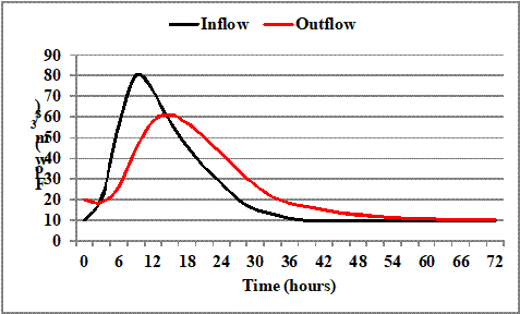
Figure 6.2: Inflow and outflow hydrographs

[2] Example 6.4 should be replaced by the following, due to a formula error in it:

Example 6.4: Using the inflow and outflow hydrographs from a channel reach given below, determine Muskingum coefficients K and x.

Time (hr)	0	4	8	12	16	20	24	28	32	36	40	44	48	52	56
Inflow (m^3/s)	42	68	116	164	194	200	192	170	150	128	106	88	74	62	54
Outflow (m^3/s)	42	39	44	65	98	133	159	174	175	168	156	140	122	106	90

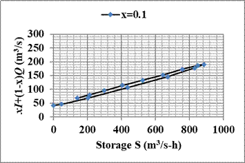
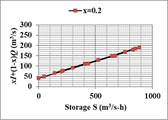
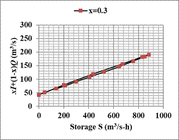
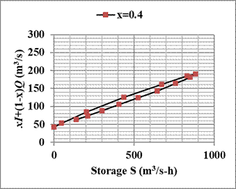
Solution: The calculation of the Muskingum coefficients (K and x) is carried out using the continuity equation (6.18). The computations are arranged in the following table. The first three columns present the inflow and outflow hydrograph data given in the example. Column 4 is the difference (I-Q) of the average inflow and outflow values at the beginning and end of the time interval and column 5 is obtained by multiplying the average of column 4 by the time interval Δt = 4 hours. The column 5 represents incremental storage ΔS in m³/s-hour. The column 6 is storage S which is obtained by accumulating the entries in column 5. Then, the next 4 columns represent the quantity {xI + (1-x)Q} for different trial values of x. The values tried are x=0.1, x=0.2, x=0.3, and x=0.4.

The plots of storage S versus the quantity {xI + (1-x)Q} are then drawn to ascertain if it shows up as a straight line. The value of x which results in this plot will be the correct value of x. As seen from the plots, the value of x=0.2 is the most appropriate as it gives a straight line with a very narrow scatter (in fact, a value between 0.2 and 0.3 would give a better straight line, but it is not really necessary to do further fine-tuning). The value of K is then obtained as the slope of the straight line in the S v/s {xI + (1-x)Q} plot corresponding to x=0.2. Selecting the storages S1=400 m³/s-hour and S2 = 800 m³/s-hour, the corresponding values of the quantity {xI + (1-x)Q} are read as 110 m³/s and 175 m³/s. Then, K = (800-400)/(175-110) = 6.15 hours. Therefore, the values of the Muskingum coefficients for the given data are K = 6.15 hours and x = 0.2.

Time	Inflow, I	Outflow	(I-Q)	ΔS=[4]*Δt	S=ΣΔS	[x I + (1 - x) Q} (m^3/s)
(Hours)	(m^3/s)	(m^3/s)	(m^3/s)	(m^3/s-h)	(m^3/s-h)	x = 0.1	x = 0.2	x = 0.3	x = 0.4
[1]	[2]	[3]	[4]	[5]	[6]	[7]	[8]	[9]	[10]
0	42	42	0.0	0	0	42.0	42.0	42.0	42.0
4	68	44	12.0	48	48	46.4	48.8	51.2	53.6
8	116	63	38.5	154	202	68.3	73.6	78.9	84.2
12	164	100	58.5	234	436	106.4	112.8	119.2	125.6
16	194	140	59.0	236	672	145.4	150.8	156.2	161.6
20	200	175	39.5	158	830	177.5	180.0	182.5	185.0
24	192	190	13.5	54	884	190.2	190.4	190.6	190.8
28	170	189	-8.5	-34	850	187.1	185.2	183.3	181.4
32	148	175	-23.0	-92	758	172.3	169.6	166.9	164.2
36	125	155	-28.5	-114	644	152.0	149.0	146.0	143.0
40	106	136	-30.0	-120	524	133.0	130.0	127.0	124.0
44	88	117	-29.5	-118	406	114.1	111.2	108.3	105.4
48	74	98	-26.5	-106	300	95.6	93.2	90.8	88.4
52	62	82	-22.0	-88	212	80.0	78.0	76.0	74.0
56	54	70	-18.0	-72	140	68.4	66.8	65.2	63.6

Chapter-7: Groundwater

The hydraulic gradient, i, has been defined as the ‘drop’ in hydraulic head per unit length. However, at several places the sign convention has not been followed. The following corrections need to be made:

[1] Page 242, in ‘hydraulic gradient along the streamline, ¶h/¶s’, there should be a negative sign

[2] Page 244, in the expressions for q_r and q_q, there should be negative signs

[3] Page 247, after Eq. (7.13), h₂−h₁ should be replaced by h₁−h₂ in all points and ‘negative’ should be changed to ‘positive’ in the third bullet

[4] Page 249, first bullet should have negative sign in the expression for i, and second bullet should have ‘negative’ in place of ‘positive’

Chapter-9: Statistical Methods in Hydrology

[1] On page 342, Last term in Eq. (9.75) should have a negative sign (- k⁵/3). This expression is an expansion of the more compact form obtained using the Wilson-Hilferty transformation as given below

K_T={[1+ k (z - k)]³ - 1}/3k

[2] On Page 343, The Log Pearson Type III table has incorrect values of K_T (and, therefore, y_T and x_T). The values should be as shown below:

T (Yrs)	z	KT	yT	xT
50	2.0537	2.0406	1.6492	44.6
100	2.3263	2.3083	1.6882	48.8
500	2.8779	2.8482	1.7669	58.5

[3] On page 346, Eq. (9.78) denominator should be 2n NOT n. Consequently, in Example 9.11 (a), Se will change to 2.638 and the values of lower and upper confidence limits will change to 37.43 mm and 47.77 mm, respectively.

[4] On page 348, for Gumbel’s distribution, correct value of Se is 6.0260 and the values of lower and upper confidence limits will change to 41.10 mm and 64.72 mm, respectively. This will change the conclusions drawn from this example.

[5] On page 348 and 349, for Log Pearson Type III distribution, correct value of K_T is 2.3083, b is 5.2183, the values of lower and upper frequency factors are 1.7723 and 3.1206, the values of lower and upper limits of y are 1.6101 and 1.8066, and the confidence limits will change to 40.75 mm and 64.06 mm, respectively.

[6] On page 360 in Q-9.10, the exceedance probabilities should be taken as 0.3, 0.1, and 0.03 in place of 0.03, 0.01, and 0.003, respectively.

[7] On page 360 in Q-9.12, ȳ should be taken as 3.6 instead of 4.6. Also, the sub-heading (d) should be read as (c).

[8] On page 360 in Q-9.13, flood magnitudes for which return periods are to be found shall be taken as 10,000 m³/s, 9,000 m³/s, 8,000 m³/s, and 5,000 m³/s, respective, instead of the values given.