0 £ lim sup_h® 0 e(h) £ 2M(w(a^m))2A,

from which, noting that A = 0 in the d (t) = o(j (t)) case, both the assertions follow, completing the proof. ð

The Oh-oh-Lemma extends an idea of [3] formalized in [2] ("Oh" -part with d(t) = t^a = j(t), f(t) = t^m, m a 0) and in [1] (f(t) = t^m); (see also [11, pp. 91, 92]). The main point of the lemma is the ease with which one is able to get certain degree of approximation results of very general orders (f(t) = e^-1/t, t^mlog t, t^m/log t; j(t) = t^a, t^a log t, t^a/(log t) ³, m a 0, any kth order modulus of smoothness w_{k(t), k < m, (for definition and many examples, see [14]) of any function in Lq(-}&yen;, &yen;), 1 &pound; q &pound; &yen; , being some examples of compatible pairs of f and j). In the present context of computerized tomography, it allows a study of window functions much more general than those satisfying a regularity condition of the type 1-F^{^(}x) ; A|x|^m, as x ® 0.

3. The tomographic spaces CT₀, CT_w, CT_j and CT_j⁰

Let CT₀ = CT₀(W^{n) denote the linear space of real-valued functions f} Î C₀(W^{n) (f defined and continuous in} R^{n, with support in} W^{n) which are essentially bandlimited in the sense that}

e(f, b) = sup_qÎSn-1 ò_{|s |&sup3;b |}s|^n-1|f^{^}(sq)|ds® 0, as b ®&yen;.

With the norm

?f?₀ = sup_qÎSn-1 ò R|s|^n-1|f^{^}(sq)|ds,

CT₀ is a complete space of which C₀&yen; (W ⁿ) is a dense subset. Since for f Î CT₀ the function

h(q) = ò_R |s|^n-1|f^{^}(sq)|ds , q Î S^n-1,

is continuous on S^n-1, the "sup" in the above is actually a "max".

A motivation for introducing the tomographic space CT₀ is the e₁-error estimate for essentially bandlimited functions. We note that CT₀ is continuously imbedded in C₀(W^{n) and that its norm comes quite close to the sup-norm; (for f radially symmetric and with f^ non-negative, the two norms in fact differ only by a factor of (2}p)^-n/2).

For a nonnegative measurable weight function w (&sup3; 1) on R^{+ = (0,} &yen;), let the space CT_&yen; (Ì CT₀) consist of functions f for which

?f?_{w = supqÎS}n-1 ò_R|s|^n-1w(|s|)|f^{^}(sq)|ds < &yen;.

Assuming the order function f of the previous section to be defined on the whole of R⁺, for f Î CT₀ and t Î R⁺, we define Peetre's K-functional Kf (t; f) with the function parameter f by

K_f(t; f) = inf_gÎCTw {?f-g?_{0 +} f(t)?g?_w}.

The w and f in the above are assumed to be tied by

4. The order functions and the filter

Let, in addition, the order function f satisfy

While studying errors due to interpolation of projection and convolveddata respectively, we assume the following additional conditions on the function u associated with the order function j :

We note here that lim_t® 0 t^mu(t) = 0, for instance, implies that (th)^m &pound; h^mu(h)j(th)/j(t) = o(j(th)), as h ® 0, for any fixed t Î (0, c]. It follows that h(J, b) &pound; c(J) e^-l(J)b = o(1/b^m) = o(j(1/b)), b ®&yen; , i.e., h(J, b) approaches zero much faster as compared to j(1/b).

In this study the order of approximation under consideration is j(1/b), as the bandwidth b ®&yen; . In the sequel the conditions on the functions F , f , j etc., imposed till now, will be assumed tobe satisfied. For a F such that 1-F^{^(}s ) = O(s^m), s® 0⁺, the choice f(t) = t^m is appropriate for orders j(t) of approximation such as t^a , t^{alog (log(1/t)), t}a/log(1/t), a < m, any moduli of smoothness w_{k(t), k < m, etc. In practice the case m = 2 is quite common (see Section 10).}

5. The intrinsic error in CBP

The intrinsic error f-W_b*f, arising due to the bandlimiting aspect of CBP, is independent of variations or refinements in the discretizations and sampling schemes.

Writing f_b^c = W_b* f = R^#(w_b* Rf), for the continuous convolution backprojection, we have f^{^}_b^c(x ) = f^{^}(x )F^{^}(x /b). Since

?f_b^c?_{w = sup}q Î_Sn-1 òR |s |^n-1w(|s |)|F ^{^}(sq /b)||f^{^}(sq )|ds ,

using F ^{^}(sq ) = 0, |s | &sup3; 1, and w(|s |) &pound; Jw(b), |s | &pound; b, and |F ^{^}(x )| &pound; B, 0 < |x | &pound; 1, for f Î CT₀ we have

?f_b^c?_w&pound; BJw(b)?f?_{0 <} &yen; ,

which, in particular, implies that f_b^cÎ CT_w. Similarly, for f Î CT_w, f_b^c Î CT_w and ?f_b^c?_w&pound; B?f?_{w. It is also clear that} ?f_b^c?&pound; ?f?_{0. Next, since,} y (|s|/b) &pound; (1/f(1/|s|)f(1/b), |s| &pound; b, and w(|s|)/w(b) &sup3; 1/J, if |s| &sup3; b, for all b sufficiently large, we have

?f-f_b^c?₀&pound; sup_qÎSn-1 {Aò_{|s |&pound; b |}s|^n-1y(|s|/b)|f^{^}(sq)|ds + (2p )^-n/2ò_{|s |b |}s|^n-1|f^{^}(sq)|ds }

&pound; max{A, (2p )^-n/2J}f(1/b)?f?_{w = D}f(1/b)?f?_{w, say.}

For any g Î CT_w,

?f-f_b^c?₀&pound; ?f-g?_{0 +} ?g-g_b^c?_{0 +} ?(g-f)_b^c?₀&pound; (1+B)?f-g?_{0 + D}f(1/b)?g?_w

&pound; max{1+B, D}(?f-g?_{0 +} f(1/b)?g?_w).

Taking the infimum over CTw, with E = max{1+B, D}, we get

Conversely, if ?f-f_b^c?_{0 = O(}d(1/b)), b ®&yen; , we have ?f-f_b^c?₀&pound; Ad(1/b), for some A and for all b sufficiently large (b &sup3; b₀, say). Then, since f_b^c Î CT_w,

Kf (t; f) = inf_gÎCTw {?f-g?_{0 +} f(t)?g?_w} &pound; inf_gÎCTw {?f- f_b^c?_{0 +} f(t)(?f_b^c-g_b^c?_w+?g_b^c?_w}

&pound; Ad (1/b) + f(t) inf_gÎCTw {BJw(b)?f-g?_{w + B}?g?_w} &pound; M[d(1/b)+(f(t)/f(1/b))K_f(1/b; f)],

where M = max{A, B, BJ}. Since this inequality is valid for all b sufficiently large and for all t, by the Oh-oh Lemma we conclude that K_f(t; f) = O(j(t)) or o(j(t)), t ® 0, according as d (t) = O(j(t)) or o(j(t)), t ® 0. Thus we have proved the following theorem.

Theorem 1 (Intrinsic error). If F , j and w satisfy the conditions (6)-(15), and f Î CT₀, then

6. An application of the Ramachandran-Lakshminarayanan filter

The ideal low-pass filter F = F ₀ given by

corresponds to the Ramachandran-Lakshminarayanan filter in R^{2. In} R^{n it corresponds to the kernel W}_b ^{= W}_b^{0 given by [9, pp. 102, 110]}

.

In this case, the two inequalities |1-F^{^(}x)| &pound; Ay (|x|), |x| < 1, and |F^{^(}x)| &pound; B, 0 &pound; |x| &pound; 1, are valid with B = 1 and for any choice of y , whatsoever. Denoting the continuous reconstruction by the Ramachandran-Lakshminarayanan filter by f_b⁰, since there holds

?f-f_b⁰?₀ = sup_qÎSn-1 ò _{|s |&sup3; b |}s |^n-1|f^{^}(sq)|ds = e(f, b),

from the Intrinsic Error Theorem we immediately get the following theorem.

Theorem 2 (Characterization of intermediate CT -spaces). Let F , j and w satisfy (6)-(15) and f Î CT₀. Then,

Corollary 3 (Intrinsic error). Let F , j and w satisfy (6)-(15) and fÎ CT₀, then, as b ® &yen; , ?f-f_b^c?₀® 0. Moreover,

7. Weighted Radon spaces R_w

Motivated by the spaces CT₀ and CT_w, consider functions g(q, s) defined on the unit cylinder Z = S^n-1&acute;R^{, for which}

?g?_w= sup_{q Î S}n-1 ò_Rw(|s|)|g^{^}(q, s)|ds < &yen; ,

where w is a nonnegative weight function on R ⁺ and g^{^}(q , s ) denotes the one-dimensional fourier transform of g(q, s), regarded as a funciton of s with q fixed. Such functions (with the usual identification of functions equal a.e.) with norm ?&times; ?w constitute our weighted radon space R w . (It may be noted that the present analysis, without forging any new tool, extends to a more general situation of ?g?w= sup ?w(&times;)g^{^}(q , &times;)?, where ?&times;? is a monotone norm, i.e., satisfying ?y?&pound; ?z? if |y(s)| &pound; |z(s)|, s ÎR^1.)

If w_{0 and} w_{1 (}&sup3; w_{0) are two weight functions, for F} ÎRw₀ we define the Peetre’s K-functional by

Kw (t; F) = inf_gÎR 1 {?F-g?w₀ + t?g?w₁}.

For b 0, let F^b be defined through F^{^b}(q, s) = F^{^}(q, s), if |s | &pound; b, and zero, otherwise. Then F^b ÎR_w if F Î R_w and moreover, ?F^b?_w&pound; ?F?_w, F Î R_w for all w , whatsoever. Let for some constant J_l, the quotient function w^{~ =} w_1/w_{0 satisfy}

w^~(|s|)/w^~(b) &pound; J_l, |s| &pound; b.

Then,

?F^b?w₁&pound; J₁w^~(b)?F?w₀,

Further, if for some constant J_r,

w^~(b)/w^~(|s|) &pound; J_r, |s| b,

then

?F-F^b?w₀ = sup_qÎSn-1ò_{|s |b}w_0(|s|)F^{^}(q, s)|ds = sup_qÎSn-1ò _|s |b w ^~(|s|)^-1w_1(|s|)F^{^}(q, s)|ds &pound; (J_r/w^~(b))?F?w₁.

Note that J_l and J_r inequalities hold for all b if

J₀ = sup_hÎ(0,1] sup_t0 w^~(th)/w^{~(t) <} &yen; ,

which we assume in the sequel.

Let a non-negaive function n on (0, c] have the following properties analogous to those of j defined earlier:

(27)

  (28)

(29)

. (30)

Let R_n = (Rw₀, Rw₁)_n be the intermediate space of g Î Rw₀ for which K_w(1/w^{~(1/t); g) = O(}n(t)), t ® 0, and R_n^{0 = (}Rw₀, Rw₁)_n^{0 of those with K}_w(1/w^{~(1/t); g) = 0(}n(t)), t ® 0. Let

e(g; b) = supq Î_Sn-1 ò_{|s |b} w_0(|s|)|g^{^}(q, s)|ds .

Then, for g Î Rw₁,

e(F; b) &pound; e(F-g; b) + e(g-g^b; b) + e((g-F)^b; b) &pound; 2?F-g?w₀ + (J_r/w^~(b))?g?w₁

&pound; max{2, J_r}[?F-g?w₀ + (J_r/w^~(b))?g?w₁],

so that

e(F; b) &pound; EK_w(1/w^{~(b); F).}

Also, since

K_w(1/w^{~(1/t); F)} &pound; inf_gÎRw1 {?F-F^b? + (1/w^~(1/t))(?(F-g)^b?+?g^b?)}

&pound; inf_gÎRw1 {e(F; b) + (1/w^~(1/t))(J₁^w~(b)?F-g?w₀ + ?g^b?w₁)}

&pound; max{1, J₁}[e(F; b) + (w^~(b)/w^~(1/t))K_w(1/w^{~(b); F)],}

applying the Oh-oh-Lemma to the function Kw (1/w ^~(1/t); F) and orders w^~(1/t) and n (t), we get the following analogue of the characterization of the intermediate CT spaces.

Theorem 4 (Characterization of intermediate Radon spaces). If w ₀, w₁ and n satisfy (26)-30),

R_n = {F Î Rw₀: e(F; b) = O(n(1/b)), b ®&yen; },

R_n^{0 = {F} Î Rw₀: e(F; b) = o(n(1/b)), b ®&yen; }.

This characterization, for appropriate choices of w₀ and w ₁, will be used in the next two sections dealing with the discretization errors due to an interpolation of the projection and the convolved data.

8. Error in the interpolation of convolved data

Suppose I_h is any interpolation of order m, for the equispaced convolved data (w_b *^{h g)(}q, s_k), k = -q, … , q, satisfying

?I_hG?_C&pound; Q_I?G?_{C, G} Î C[-1, 1], (31)

?I_hG-G?_C&pound; C_Ih^m?G^(m)?_{C, G} Î C^m[-1, 1], (32)

where ?&times;?_{C denotes the sup-norm on the interval [-1, 1], C}^m_{[-1, 1] is the space of m-times continuously differentiable functions on [-1, 1] and where QI and CI are independent of h. An appropriate example of such an Ih is the m-point central difference interpolation. For the standard two-point linear interpolation used in most CBP applications we have m = 2.}

Using [9, p. 58]

(wb *^{h g)^(}q , s) = (2p)^1/2w_b^{^}(s)S_lÎZg^{^}₍q, s-(2pl/h)),

and with D denoting the partial differentiation &para;/&para;s, since |F^{^(}x)| &pound; B, 0 &pound; |x| &pound; 1, and w_b^{^}(s) = 0 for |s| b, we have

|D^m(w_b *^{h g)(}q, s)| &pound; ò_{[-b,b] |}s|^m|w_b^{^}(s)|S_lÎZ|g^{^}₍q, s-(2pl/h))|ds

&pound; (2p )^1/2-n((1/2)B)ò_{[-b,b] |}s|^m+n-1S_lÎZ|g^{^}₍q, s-(2pl/h))|ds .

Putting

(E_hw_b *^{h g)(}q, s) = (I_hw_b*^{h g - w}_b*^{h g)(}q, s),

and, using b &pound; p/h,

?E_hw_b*^{h g}? = sup_qÎSn-1?E_hw_b*^{h g(}q, .)?_C&pound; sup_qÎSn-1 C_Ih^m?D^mw_b*^{h g(}q, .)?_C

&pound; C_Ih^m sup_qÎSn-1ò_R |s|^m|(w_b *^{h g^(}q, s)|ds

&pound; (2p)^1/2-n((1/2)B) sup_qÎSn-1 C_Ih^mò_R^|s|^m+n-1|g^{^}(q, s)|ds .

From this, with w₁₍s) = max{|s|^m+n-1, 1}, there follows

?E_hw_b *^{h g}? &pound;(2p)^1/2-n((1/2)B)?g?w₁.

With w₀₍s) = max{|s|^n-1, 1}, w^~(s) = max{|s|^m, 1} and we have

?E_hw_b *^{h g}? &pound;Q_I?w_b *^{h g}?_C&pound;Q_I(2p)^1/2-n((1/2)B)?g?w₀.

It follows that for a general g,

?E_hw_b *^{h g}? &pound;inf_GÎR1 {?E_hw_b *^{h (g-G)}? + ?E_hw_b *^{h G}?}

&pound; max {Q_I, C_I}(2p)^1/2-n((1/2)B) inf_GÎR1 {?g-G?w₀ + h^m?G?w₁}

= max {Q_I, C_I}(2p)^1/2-n((1/2)B)K_w(h^m; g).

Next,

sup_qÎSn-1ò_{|s |b}w_0(|s|)|g^{^}(q, s)|ds

= (2p)^(n-1)/2?f-f^b?₀

&pound; inf_FÎCTw (2p)^(n-1)/2{?(f-F)-(f-F^b)?_{0 +} ?F-F^b?_0}

&pound; inf_FÎCTw (2p)^(n-1)/2{?f-F?_{0 + J}f(1/b)?F?_w}

&pound; inf_FÎCTw (2p)^(n-1)/2J{?f-F?_{0 +} f(1/b)?F?_w}

&pound; (2p)^(n-1)/2JKf(1/b; f).

Hence, if f Î CT_w,

sup_qÎSn-1ò_{|s |b}w_0(|s|)|g^{^}(q, s)|ds = O(j(1/b)), b ® &yen; .

Using lim_t® 0 t^mu(t) = 0, this and the theorem on the characterization of intermediate Radon spaces imply that K_w(t^m; g) = O(j(t)), t ® 0. Hence, from the K_w -estimate of E_h in the above, there follows ?I_h(w_b*_g)-wb*_g? = O(j(h)), so that finally we have e_I = |R_p^#(I_h(w_b *^{h g)-w}_b *^{h g)| = O(}j(1/b)), showing that the net contribution of the error due to the interpolation of the convolved data is of the order of j(1/b).

Similarly, e_I = o(j(1/b)), for f Î CT_j^{0, and e}_I ^{= o(1), for f} Î CT₀ and m 0 (for the details of the reasoning, see the next section), as b ® &yen; . Thus we have proved the following theorem:

Theorem 5 (Error in the interpolation of convolved data). If the assumptions (1), (2), (6)-(15), (17) and (31), (32) hold,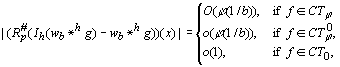

(33)

uniformly in x ÎW ⁿ

9. Error in the interpolationof projection data

Let the minimum spacing h_m and the maximum spacing h_M between consecutive local interpolation data points satisfy b &pound; h_m/h_M, where b is a certain (positive) constant. With the largest of the data spacings denoted by h (assumed to be of the order of h, i.e., h/h &pound; C for some constant C), let the projection data interpolation operator J_h be of order l:

J_h g(q, s) = S_{1&pound; k&pound; l lk(s)g(}q, z_k),

l_k(s) = P_{1&pound; j(&sup1; k)&pound; l ((s-zj)/(zk-zj)), k = 1, … , l,}

Based on appropritate local nodes z1, z2, … , zk, provides an lth-order interpolation.

We take g(q, s) as the projection data for f. Putting

(E_h g)(q, s) = (J_h g – g)(q, s) and ?E_h g? = sup_qÎSn-1?E_h g(q, &times;)?_C,

we have

?E_h g? &pound; (2p)^-1/2C_jh^{l sup}_qÎSn-1ò_R |s|^l |g^{^}(q, s)|ds ,

from which, if we take w_l(s) = max{|s|^l, 1}, there follows

?E_h g? &pound; (2p)^-1/2C_jh^l?g?w_l,

Also, with w₀₍s) = 1, for some constant H₀ (depending on b ),

?E_h g? &pound; H₀?g?w₀.

Then, w^{^(}s) = w₁₍s)/w₀₍s) = w₁₍s) = max{|s|^l, 1} and hence, for any g Î R_0,

?E_h g? &pound; inf_GÎR1 {?E_h (g-G)? + ?E_h (g-G)?}

&pound; max {H₀, (2p)^-1/2C_J} inf_GÎR1 {?E_h (g-G)?w₀ + h^l ?G?w₁}

= max {H₀, (2p)^-1/2C_J} K_w(h^{l; g).}

Since, g^(q, s) = (2p )^(n-1)/2f^{^}(sq), by the projection theorem, for f Î CT₀, we have

sup_qÎSn-1ò_{|s |b |g}^{^}₍q, s)|ds&pound; (2p)^(n-1)/2?f?_0/b^n-1

and, if f Î CT_w,

sup_qÎSn-1ò_{|s |b |g}^{^}₍q, s)|ds&pound; Jb^-(n-1)f(1/b) sup_qÎSn-1ò_{|s |b (|}s|^n-1/f(1/|s|)) |g^{^}(q, s)|ds

&pound; Jb^-(n-1)f(1/b) (2p)^(n-1)/2?f?_w.

It follows that for any f Î CT₀,

e(g; b) = sup_qÎSn-1ò_{|s |b |g}^{^}₍q, s)|ds = (2p)^(n-1)/2?f - f^b?w₀, say,

&pound; (2p)^(n-1)/2 inf_fÎCTw {?(f-F)-(f-F)^b?w₀ + ?F-F^b?w₀}

&pound; inf_fÎCTw (2p)^(n-1)/2 b^-(n-1) {?f-F?_{0 + J}f(1/b)?F-F^b?_w}

&pound; inf_fÎCTw (2p)^(n-1)/2 b^-(n-1) J{?f-F?_{0 +} f(1/b)?F-F^b?_w}

&pound; (2p)^(n-1)/2 b^-(n-1) JK_f(1/b; f).

With w(s) = w₁(s), bh = Jp , J Î (0, 1], and assuming that J is such that

s_{w = |w(0)| + 2}S_{1&pound; j<&yen; |w(j}Jp)| < &yen; , (36)

using (1) and the positivity of the a_{pj’s, we have}

eJ = |Rp^#_(Ih{wb *^{h (J}_h g - g)})| &pound; S_{1&pound; j&pound; p} a_pjQI ?E_h g?hS_{-q&pound;l&pound;q |wb(lh)|}

? |S^n-1| bⁿQ_Ihs_w?Eh g?.

At this point we may note that if N denotes the order of magnitude of an extraneous noise N(q_{j, s) in the projection data for a single projection view} q_j, the worst-case reconstruction error at a point is of order a_pjhbⁿs_{w,qN, where} s_{w,q= |w(0)| + 2}S_{1&pound;j&pound;q|w(j}Jp)|. Thus s_{w provides a useful measure of a filter’s sensitivity to noise. Since, for the p and q in practice, approximately p = cq}^n-1_{, c =} p^{n-1/(n-1)! [9, p. 70], and the quadrature coefficients} a_pj are practically of the order 1/p of magnitude, the noise propagation due to a single view is of order O(Ns_w,q).

If f Î CT_j , e(g; b) = O(b^-(n-1)j(1/b)). Taking n(t) = t^n-1j(t), and using lim_t®0 t^l-n+1u(t) = 0, from the theorem on the characterization of intermediate Radon spaces, we have g Î R_n and consequently, since h = O(h) = O(1/b), e_J = O(j(1/b)). Similarly, f Î CT_j^{0 implies that e}_J ^{= o(}j(1/b)). Moreover, if f Î CT₀, e(g; b) = o(b^-(n-1)) and then with j = 1, since for l n-1, lim_t® 0t^l-n+1 = 0, we have e_J = 0(1), b ®&yen; . Thus we have proved the following theorem.

Theorem 6 (Error in the interpolation of projection data). If (1), (2), (6)-16), (31), (32) and (34)-(36) hold and h = O(1/b), then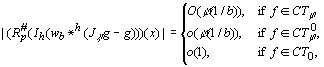

(37)

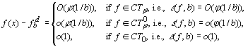
uniformly in x ÎW ⁿ