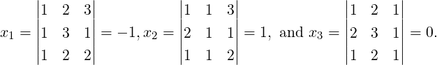
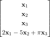
Example 2.1.1. Let us look at some examples of linear systems.
-
1.
- Suppose a,b ∈ ℝ. Consider the system ax = b in the variable x. If
-
(a)
- a≠0 then the system has a unique solution x =
 .
.
-
(b)
- a = 0 and
-
i.
- b≠0 then the system has no solution.
-
ii.
- b = 0 then the system has infinite number of solutions, namely all x ∈ ℝ.
-
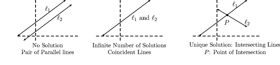
2.
- Consider a linear system with 2 equations in 2 variables. The equation ax + by = c in the
variables x and y represents a line in ℝ2 if either a≠0 or b≠0. Thus the solution set of the
system
 is given by the points of intersection of the two lines (see Figure 2.1 for illustration of different
cases).
is given by the points of intersection of the two lines (see Figure 2.1 for illustration of different
cases).
-
(a)
- Unique Solution
x - y = 3 and 2x + 3y = 11. The unique solution is [x,y]T = [4,1]T .
Observe that in this case, a1b2 - a2b1≠0.
-
(b)
- Infinite Number of Solutions
x + 2y = 1 and 2x + 4y = 2. As both equations represent the same line, the
solution set is [x,y]T = [1 - 2y,y]T = [1,0]T + y[-2,1]T with y arbitrary. Observe
that
-
i.
- a1b2 - a2b1 = 0,a1c2 - a2c1 = 0 and b1c2 - b2c1 = 0.
-
ii.
- the vector [1,0]T corresponds to the solution x = 1,y = 0 of the given system.
-
iii.
- the vector [-2,1]T corresponds to the solution x = -2,y = 1 of the system
x + 2y = 0,2x + 4y = 0.
-
(c)
- No Solution
x + 2y = 1 and 2x + 4y = 3. The equations represent a pair of parallel lines and hence
there is no point of intersection. Observe that in this case, a1b2 - a2b1 = 0 but
a1c2 - a2c1≠0.
-
3.
- As a last example, consider 3 equations in 3 variables.
A linear equation ax + by + cz = d represents a plane in ℝ3 provided [a,b,c]≠[0,0,0]. Here, we
have to look at the points of intersection of the three given planes. It turns out that there are
seven different ways in which the three planes can intersect. We present only three ways which
correspond to different cases.

 DRAFT
DRAFT
-
(a)
- Unique Solution
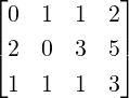
Consider the system x+y+z = 3,x+4y+2z = 7 and 4x+10y-z = 13. The unique
solution to this system is [x,y,z]T = [1,1,1]T , i.e., the three planes intersect
at a point.
-
(b)
- Infinite Number of Solutions
Consider the system x + y + z = 3,x + 2y + 2z = 5 and 3x + 4y + 4z = 11. The solution set
is [x,y,z]T = [1,2 - z,z]T = [1,2,0]T + z[0,-1,1]T , with z arbitrary. Observe the
following:
-
i.
- Here, the three planes intersect in a line.
-
ii.
- The vector [1,2,0]T corresponds to the solution x = 1,y = 2 and z = 0 of the
linear system x + y + z = 3,x + 2y + 2z = 5 and 3x + 4y + 4z = 11. Also, the
vector [0,-1,1]T corresponds to the solution x = 0,y = -1 and z = 1 of the
linear system x + y + z = 0,x + 2y + 2z = 0 and 3x + 4y + 4z = 0.
-
(c)
- No Solution
The system x + y + z = 3,2x + 2y + 2z = 5 and 3x + 3y + 3z = 3 has no solution. In
this case, we have three parallel planes. The readers are advised to supply the
proof.
Before we start with the general set up for the linear system of equations, we give different
interpretations of the examples considered above.
Example 2.1.2.
-
1.
- Recall Example 2.1.1.2a, where we have verified that the solution of the linear system x-y = 3
and 2x + 3y = 11 equals [4,1]T . Now, observe the following:
-
(a)
- The solution [4,1]T corresponds to the point of intersection of the corresponding two
lines.
-
(b)
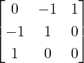
- Using matrix multiplication the linear system equals Ax = b, where A =
![[ ]
1 - 1
2 3](LA262x.png) ,
,

 DRAFT
x =
DRAFT
x = ![[ ]
x
y](LA263x.png) and b =
and b = ![[ ]
3
11](LA264x.png) . So, the solution is x = A-1b =
. So, the solution is x = A-1b = 
![[ ]
3 1
- 2 1](LA266x.png)
![[ ]
3
11](LA267x.png) =
= ![[ ]
4
1](LA268x.png) .
.
-
(c)
- Re-writing Ax = b as
![[ ]
1
2](LA271x.png) x+
x+![[ ]
- 1
3](LA272x.png) y =
y = ![[ ]
3
11](LA273x.png) gives us 4⋅(1,2)+1⋅(-1,3) = (3,11).
This corresponds to addition of vectors in the Euclidean plane.
gives us 4⋅(1,2)+1⋅(-1,3) = (3,11).
This corresponds to addition of vectors in the Euclidean plane.
-
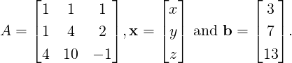
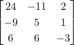
2.
- Recall Example 3.3a, where the point of intersection of the three planes is the point (1,1,1) in
the Euclidean space. Note that in matrix notation, the system reduces to Ax = b,
where
 Then
Then
-
(a)
- x =
 = A-1
b =
= A-1
b = 
 =
=  .
.
-
(b)
- 1 ⋅ (1,1,4) + 1 ⋅ (1,4,10) + 1 ⋅ (1,2,-1) = (3,5,13). This corresponds to addition of
vectors in the Euclidean space.
Thus, there are three ways of looking at the linear system Ax = b, where, as the name suggests, one of
the ways is looking at the point of intersection of planes, the other is the vector sum approach and the
third is the matrix multiplication approach. All of three approaches are important as they give
different insight to the study of matrices. After this chapter, we will see that the last two
interpretations form the fundamentals of linear algebra.
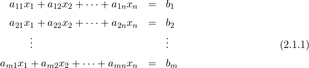
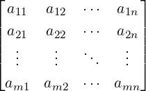
Definition 2.1.3. [Linear System] A system of m linear equations in n variables x1,x2,…,xn
is a set of equations of the form

 DRAFT
DRAFT
where for 1
≤ i ≤ m and 1
≤ j ≤ n;
aij,bi ∈ ℝ. Linear System (
2.1.1) is called
homogeneous if
b1 = 0 =
b2 =

=
bm and
non-homogeneous, otherwise.
Remark 2.1.5. Consider the linear system Ax = b, where A ∈ Mm,n(ℂ), b ∈ Mm,1(ℂ) and
x ∈ Mn,1(ℂ). If [Ab] is the augmented matrix and xT = [x1,…,xn] then,
-
1.
- for j = 1,2,…,n, the variable xj corresponds to the column ([Ab])[:,j].

 DRAFT
DRAFT
-
2.
- the vector b = ([Ab])[:,n + 1].
-
3.
- for i = 1,2,…,m, the ith equation corresponds to the row ([Ab])[i,:].
Definition 2.1.7. [Consistent, Inconsistent] Consider a linear system Ax = b. Then, this
linear system is called consistent if it admits a solution and is called inconsistent if it admits
no solution. For example, the homogeneous system Ax = 0 is always consistent as 0 is a solution
whereas, verify that the system x + y = 2,2x + 2y = 3 is inconsistent.
Definition 2.1.8. [Associated Homogeneous System] Consider a linear system Ax = b.
Then, the corresponding linear system Ax = 0 is called the associated homogeneous system.
0 is always a solution of the associated homogeneous system.
The readers are advised to supply the proof of the next theorem that gives information about the
solution set of a homogeneous system.

 DRAFT
Theorem 2.1.9. Consider a homogeneous linear system Ax = 0.
DRAFT
Theorem 2.1.9. Consider a homogeneous linear system Ax = 0.
-
1.
- Then, x = 0, the zero vector, is always a solution, called the trivial solution.
-
2.
- Let u≠0 be a solution of Ax = 0. Then, y = cu is also a solution, for all c ∈ ℂ. A nonzero
solution is called a non-trivial solution. Note that, in this case, the system Ax = 0 has
an infinite number of solutions.
-
3.
- Let u1,…,uk be solutions of Ax = 0. Then, ∑
i=1kaiui is also a solution of Ax = 0, for
each choice of ai ∈ ℂ,1 ≤ i ≤ k.
Remark 2.1.10.
-
1.
- Let A =
![[ ]
1 1
1 1](LA295x.png) . Then, x =
. Then, x = ![[ ]
1
- 1](LA296x.png) is a non-trivial solution of Ax = 0.
is a non-trivial solution of Ax = 0.
-
2.
- Let u≠v be solutions of a non-homogeneous system Ax = b. Then, xh = u-v is a solution
of the associated homogeneous system Ax = 0. That is, any two distinct solutions of
Ax = b differ by a solution of the associated homogeneous system Ax = 0. Or equivalently,
the solution set of Ax = b is of the form, {x0 + xh}, where x0 is a particular solution of
Ax = b and xh is a solution of the associated homogeneous system Ax = 0.
Exercise 2.1.11.
-
1.
- Consider a system of 2 equations in 3 variables. If this system is consistent then how many
solutions does it have?

 DRAFT
DRAFT
-
2.
- Give a linear system of 3 equations in 2 variables such that the system is inconsistent
whereas it has 2 equations which form a consistent system.
-
3.
- Give a linear system of 4 equations in 3 variables such that the system is inconsistent
whereas it has three equations which form a consistent system.
-
4.
- Let Ax = b be a system of m equations in n variables, where A ∈ Mm,n(ℂ).
-
(a)
- Can the system, Ax = b have exactly two distinct solutions for any choice of m and
n? Give reasons for your answer. Give reasons for your answer.
-
(b)
- Can the system, Ax = b have only a finitely many (greater than 1) solutions for any
choice of m and n? Give reasons for your answer.
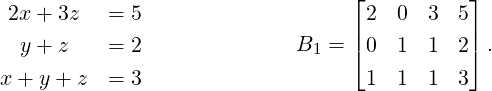
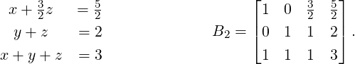
Example 2.1.12. Solve the linear system y + z = 2,2x + 3z = 5,x + y + z = 3.
Solution: Let B0 = [Ab], the augmented matrix. Then, B0 =  . We now systematically
proceed to get the solution.
. We now systematically
proceed to get the solution.
-
1.
- Interchange 1-st and 2-nd equations (interchange B0[1,:] and B0[2,:] to get B1).
-
2.
- In the new system, multiply 1-st equation by
 (multiply B1[1,:] by
  to get B2).
-
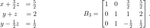
3.
- In the new system, replace 3-rd equation by 3-rd equation minus 1-st equation (replace
B2[3,:] by B2[3,:] - B2[1,:] to get B3).
-
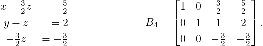
4.
- In the new system, replace 3-rd equation by 3-rd equation minus 2-nd equation (replace
B3[3,:] by B3[3,:] - B3[2,:] to get B4).

 DRAFT
DRAFT
-
5.
- In the new system, multiply 3-rd equation by
 (multiply B4[3,:] by
  to get B5).
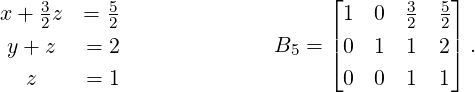
The last equation gives z = 1. Using this, the second equation gives y = 1. Finally, the first
equation gives x = 1. Hence, the solution set is {[x,y,z]T |[x,y,z] = [1,1,1]}, a unique
solution.
In Example 2.1.12, observe how each operation on the linear system corresponds to a similar
operation on the rows of the augmented matrix. We use this idea to define elementary row operations
and the equivalence of two linear systems.
Definition 2.1.13. [Elementary Row Operations] Let A ∈ Mm,n(ℂ). Then, the elementary row
operations are
-
1.
- Eij: Interchange the i-th and j-th rows, namely, interchange A[i,:] and A[j,:].
-
2.
- Ek(c) for c≠0: Multiply the k-th row by c, namely, multiply A[k,:] by c.
-
3.
- Eij(c) for c≠0: Replace the i-th row by i-th row plus c-times the j-th row, namely, replace
A[i,:] by A[i,:] + cA[j,:].

 DRAFT
DRAFT
Definition 2.1.14. [Row Equivalent Matrices] Two matrices are said to be row equivalent
if one can be obtained from the other by a finite number of elementary row operations.
Definition 2.1.15. [Row Equivalent Linear Systems] The linear systems Ax = b and
Cx = d are said to be row equivalent if their respective augmented matrices, [Ab] and [Cd],
are row equivalent.
Thus, note that the linear systems at each step in Example 2.1.12 are row equivalent to
each other. We now prove that the solution set of two row equivalent linear systems are
same.
Lemma 2.1.16. Let Cx = d be the linear system obtained from Ax = b by application of a
single elementary row operation. Then, Ax = b and Cx = d have the same solution set.
Proof. We prove the result for the elementary row operation Ejk(c) with c≠0. The reader is advised to
prove the result for the other two elementary operations.
In this case, the systems Ax = b and Cx = d vary only in the jth equation. So, we
need to show that y satisfies the jth equation of Ax = b if and only if y satisfies the jth
equation of Cx = d. So, let yT = [α1,…,αn]. Then, the jth and kth equations of Ax = b are
aj1α1 +  + ajnαn = bj and ak1α1 +
  + aknαn = bk. Therefore, we see that αi’s satisfy
Also, by definition the jth equation of Cx = d equals Therefore, using Equation (2.1.2), we see that yT = [α1,…,αn] is also a solution for Equation (2.1.3).
Now, use a similar argument to show that if zT = [β1,…,βn] is a solution of Cx = d then it is also a
solution of Ax = b. Hence, the required result follows. _
The readers are advised to use Lemma 2.1.16 as an induction step to prove the next
result.
Theorem 2.1.17. Let Ax = b and Cx = d be two row equivalent linear systems. Then, they
have the same solution set.
In the previous section, we saw that two row equivalent linear systems have the same solution set.
Sometimes it helps to imagine an elementary row operation as left multiplication by a suitable matrix.
In this section, we will try to understand this relationship and use them to obtain results for linear
system. As special cases, we also obtain results that are very useful in the study of square
matrices.

 DRAFT
DRAFT
Definition 2.2.1. [Elementary Matrix] A matrix E ∈ Mn(ℂ) is called an elementary
matrix if it is obtained by applying exactly one elementary row operation to the identity matrix
In.
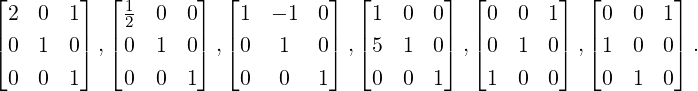
Remark 2.2.2. The elementary matrices are of three types and they correspond to elementary row
operations.
-
1.
- Eij: Matrix obtained by applying elementary row operation Eij to In.
-
2.
- Ek(c) for c≠0: Matrix obtained by applying elementary row operation Ek(c) to In.
-
3.
- Eij(c) for c≠0: Matrix obtained by applying elementary row operation Eij(c) to In.
When an elementary matrix is multiplied on the left of a matrix A, it gives the same result as that of
applying the corresponding elementary row operation on A.
Remark 2.2.5. Observe that
-
1.
- (Eij)-1 = Eij as EijEij = I = EijEij.

 DRAFT
DRAFT
-
2.
- Let c≠0. Then, (Ek(c))-1 = Ek(1∕c) as Ek(c)Ek(1∕c) = I = Ek(1∕c)Ek(c).
-
3.
- Let c≠0. Then, (Eij(c))-1 = Eij(-c) as Eij(c)Eij(-c) = I = Eij(-c)Eij(c).
Thus, each elementary matrix is invertible. Also, the inverse is an elementary matrix of
the same type.
Proposition 2.2.6. Let A and B be two row equivalent matrices. Then, prove that B =
E1 EkA, for some elementary matrices E1,…,Ek.
Proof. By definition of row equivalence, the matrix B can be obtained from A by a finite number of
elementary row operations. But by Remark 2.2.2, each elementary row operation on A
corresponds to left multiplication by an elementary matrix to A. Thus, the required result
follows. _
We now give an alternate prove of Theorem 2.1.17. To do so, we state the theorem once
again.
Theorem 2.2.7. Let Ax = b and Cx = d be two row equivalent linear systems. Then, they
have the same solution set.
Proof. Let E1,…,Ek be the elementary matrices such that E1 Ek[Ab] = [Cd]. Put E = E1
 Ek.
Then, by Remark 2.2.5
Ek.
Then, by Remark 2.2.5
 | (2.2.1) |

 DRAFT
DRAFT
Now assume that Ay = b holds. Then, by Equation (2.2.1)
 | (2.2.2) |
On the other hand if Cz = d holds then using Equation (2.2.1), we have
 | (2.2.3) |
Therefore, using Equations (2.2.2) and (2.2.3) the required result follows. _
The following result is a particular case of Theorem 2.2.7.
Corollary 2.2.8. Let A and B be two row equivalent matrices. Then, the systems Ax = 0 and
Bx = 0 have the same solution set.
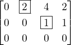
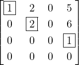
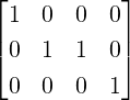
Definition 2.2.10. [Pivot/Leading Entry] Let A be a nonzero matrix. Then, in each nonzero
row of A, the left most nonzero entry is called a pivot/leading entry. The column containing
the pivot is called a pivotal column. If aij is a pivot then we denote it by aij. For example,
the entries a12 and a23 are pivots in A = 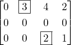 . Thus, columns 2 and 3 are pivotal
columns.
. Thus, columns 2 and 3 are pivotal
columns.
Definition 2.2.11. [Row Echelon Form] A matrix is in row echelon form (REF) (ladder
like)
-
1.
- if the zero rows are at the bottom;
-
2.
- if the pivot of the (i + 1)-th row, if it exists, comes to the right of the pivot of the i-th
row.
-
3.
- if the entries below the pivot in a pivotal column are 0.
Definition 2.2.13. [Row-Reduced Echelon Form (RREF)] A matrix C is said to be in
row-reduced echelon form (RREF)
-
1.
- if C is already in echelon form,
-
2.
- if the pivot of each nonzero row is 1,
-
3.
- if every other entry in each pivotal column is zero.
A matrix in RREF is also called a row-reduced echelon matrix.
Let A ∈ Mm,n(ℂ). We now present an algorithm, commonly known as the Gauss-Jordan
Elimination (GJE), to compute the RREF of A.
-
1.
- Input: A.
-
2.
- Output: a matrix B in RREF such that A is row equivalent to B.
-
3.
- Step 1: Put ‘Region’ = A.
-
4.
- Step 2: If all entries in the Region are 0, STOP. Else, in the Region, find the leftmost
nonzero column and find its topmost nonzero entry. Suppose this nonzero entry is aij = c
(say). Box it. This is a pivot.
-
5.
- Step 3: Interchange the row containing the pivot with the top row of the region. Also,
make the pivot entry 1 by dividing this top row by c. Use this pivot to make other entries
in the pivotal column as 0.
-
6.
- Step 4: Put Region = the submatrix below and to the right of the current pivot. Now,
go to step 2.
Important: The process will stop, as we can get at most min{m,n} pivots.
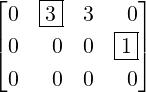
Example 2.2.15. Apply GJE to 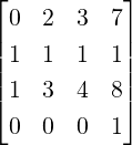
-
1.
- Region = A as A≠0.
-
2.
- Then, E12A =
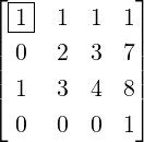 . Also, E31(-1)E12A =
 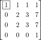 = B (say).

 DRAFT
DRAFT
-
3.
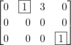
- Now, Region =
 ≠0. Then, E
2(
≠0. Then, E
2( )B =
)B = 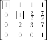 = C(say). Then,
E12(-1)E32(-2)C =
= C(say). Then,
E12(-1)E32(-2)C = 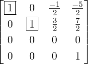 = D(say).
-
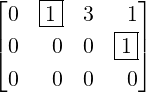
4.
- Now, Region =
![[ ]
0 0
0 1](LA378x.png) . Then, E34D =
. Then, E34D = 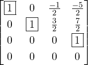 . Now, multiply on the left
by E13(
. Now, multiply on the left
by E13( ) and E23(
 ) to get
 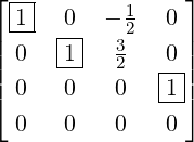 , a matrix in RREF. Thus, A is row
equivalent to F, where F = RREF(A) =
, a matrix in RREF. Thus, A is row
equivalent to F, where F = RREF(A) = 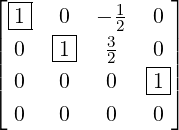 .
.
The proof of the next result is beyond the scope of this book and hence is omitted.
Theorem 2.2.17. Let A and B be two row equivalent matrices in RREF. Then A = B.
As an immediate corollary, we obtain the following important result.
Corollary 2.2.18. The RREF of a matrix A is unique.
Proof. Suppose there exists a matrix A with two different RREFs, say B and C. As the RREFs are
obtained by left multiplication of elementary matrices, there exist elementary matrices E1,…,Ek and
F1,…,Fℓ such that B = E1 EkA and C = F1
 FℓA. Let E = E1
 Ek and F = F1
 Fℓ. Thus,
B = EA = EF-1C.
Fℓ. Thus,
B = EA = EF-1C.
As inverse of an elementary matrix is an elementary matrix, F-1 is a product of elementary
matrices and hence, B and C are row equivalent. As B and C are in RREF, using Theorem 2.2.17,
B = C. _
Remark 2.2.19. Let A ∈ Mm,n(ℂ).

 DRAFT
DRAFT
-
1.
- Then, by Corollary 2.2.18, it’s RREF is unique.
-
2.
- Let A ∈ Mm,n(ℂ). Then, the uniqueness of RREF implies that RREF(A) is independent
of the choice of the row operations used to get the final matrix which is in RREF.
-
3.
- Let B = EA, for some elementary matrix E. Then, RREF(A) = RREF(B).
Proof. Let E1,…,Ek and F1,…,Fℓ be elementary matrices such that RREF(A) =
E1 EkA and RREF(B) = F1
 FℓB. Then,
 Thus, the matrices RREF(A) and RREF(B) are row equivalent. Since they are also in
RREF by Theorem 2.2.17, RREF(A) = RREF(B). _
Thus, the matrices RREF(A) and RREF(B) are row equivalent. Since they are also in
RREF by Theorem 2.2.17, RREF(A) = RREF(B). _
-
4.
- Then, there exists an invertible matrix P, a product of elementary matrices, such that
PA = RREF(A).
Proof. By definition, RREF(A) = E1 EkA, for certain elementary matrices E1,…,Ek.
Take P = E1
EkA, for certain elementary matrices E1,…,Ek.
Take P = E1 Ek. Then, P is invertible (product of invertible matrices is invertible) and
PA = RREF(A). _
Ek. Then, P is invertible (product of invertible matrices is invertible) and
PA = RREF(A). _
-
5.
- Let F = RREF(A) and B = [A[:,1],…,A[:,s]], for some s ≤ n. Then,
![RREF (B ) = [F [:,1],...,F [:,s]].](LA400x.png)
Proof. By Remark 2.2.19.4, there exist an invertible matrix P, such that

 DRAFT
DRAFT
![F = PA = [P A[:,1],...,PA [:,n]] = [F[:,1],...,F[:,n ]].](LA401x.png) Thus, PB = [PA[:,1],…,PA[:,s]] = [F[:,1],…,F[:,s]]. As F is in RREF, it’s first s
columns are also in RREF. Hence, by Corollary 2.2.18, RREF(PB) = [F[:,1],…,F[:,s]].
Now, a repeated use of Remark 2.2.19.3 gives RREF(B) = [F[:,1],…,F[:,s]]. Thus, the
required result follows. _
Thus, PB = [PA[:,1],…,PA[:,s]] = [F[:,1],…,F[:,s]]. As F is in RREF, it’s first s
columns are also in RREF. Hence, by Corollary 2.2.18, RREF(PB) = [F[:,1],…,F[:,s]].
Now, a repeated use of Remark 2.2.19.3 gives RREF(B) = [F[:,1],…,F[:,s]]. Thus, the
required result follows. _
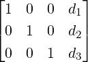
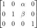
Example 2.2.20. Consider a linear system Ax = b, where A ∈ M3(ℂ) and A[:,1]≠0
(recall Example 2.1.1.3). Then, verify that the 7 different choices for [Cd] = RREF([Ab])
are
-
1.
-
 . Here, Ax = b is consistent. The unique solution equals
  =
=  .
.
-
2.
-
 ,
,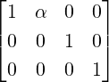 or
or 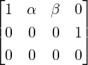 . Here, Ax = b is inconsistent for
any choice of α,β as RREF([Ab]) has a row of [0001]. This corresponds to solving
0 ⋅ x + 0 ⋅ y + 0 ⋅ z = 1, an equation which has no solution.
. Here, Ax = b is inconsistent for
any choice of α,β as RREF([Ab]) has a row of [0001]. This corresponds to solving
0 ⋅ x + 0 ⋅ y + 0 ⋅ z = 1, an equation which has no solution.
-
3.
-
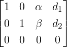 ,
,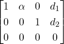 or
or 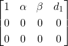 . Here, Ax = b is consistent and has
infinite number of solutions for every choice of α,β as RREF([Ab]) has no row of
the form [0001].
. Here, Ax = b is consistent and has
infinite number of solutions for every choice of α,β as RREF([Ab]) has no row of
the form [0001].

 DRAFT
Proposition 2.2.21. Let A ∈ Mn(ℂ). Then, A is invertible if and only if RREF(A) = In.
That is, every invertible matrix is a product of elementary matrices.
DRAFT
Proposition 2.2.21. Let A ∈ Mn(ℂ). Then, A is invertible if and only if RREF(A) = In.
That is, every invertible matrix is a product of elementary matrices.
Proof. If RREF(A) = In then In = E1 EkA, for some elementary matrices E1,…,Ek. As Ei’s are
invertible, E1-1 = E2
EkA, for some elementary matrices E1,…,Ek. As Ei’s are
invertible, E1-1 = E2 EkA, E2-1E1-1 = E3
 EkA and so on. Finally, one obtains
A = Ek-1
EkA and so on. Finally, one obtains
A = Ek-1 E1-1. A similar calculation now gives AE1
 Ek = In. Hence, by definition of
invertibility A-1 = E1
Ek = In. Hence, by definition of
invertibility A-1 = E1 Ek.
Ek.
Now, let A be invertible with B = RREF(A) = E1 EkA, for some elementary matrices E1,…,Ek.
As A and Ei’s are invertible, the matrix B is invertible. Hence, B doesn’t have any zero row. Thus, all
the n rows of B have pivots. Therefore, B has n pivotal columns. As B has exactly n
columns, each column is a pivotal column and hence B = In. Thus, the required result
follows. _
EkA, for some elementary matrices E1,…,Ek.
As A and Ei’s are invertible, the matrix B is invertible. Hence, B doesn’t have any zero row. Thus, all
the n rows of B have pivots. Therefore, B has n pivotal columns. As B has exactly n
columns, each column is a pivotal column and hence B = In. Thus, the required result
follows. _
As a direct application of Proposition 2.2.21 and Remark 2.2.19.3 one obtains the
following.
Theorem 2.2.22. Let A ∈ Mm,n(ℂ). Then, for any invertible matrix S, RREF(SA) =
RREF(A).
Proof. Using matrix product,
![[ ] [ ]
A -1C = A -1A A-1B = In A- 1B .](LA426x.png) As
As
![[ ]
In A -1B](LA427x.png) is in RREF, by Remark 2.2.19.1, RREF(C) =
is in RREF, by Remark 2.2.19.1, RREF(C) = ![[ ]
In A- 1B](LA428x.png) .
.

 DRAFT
DRAFT
For the second part, note that the matrix X = ![[ ]
A -1 0
- BA -1 In](LA429x.png) is an invertible matrix.
Thus, by Proposition 2.2.21, X is a product of elementary matrices. Now, verify that
XD =
is an invertible matrix.
Thus, by Proposition 2.2.21, X is a product of elementary matrices. Now, verify that
XD = ![[ ]
In
0](LA430x.png) . As
. As ![[ ]
In
0](LA431x.png) is in RREF, a repeated application of Remark 2.2.19.1 gives the required
result. _
is in RREF, a repeated application of Remark 2.2.19.1 gives the required
result. _
As an application of Proposition 2.2.23, we have the following observation.
Let A ∈ Mn(ℂ). Suppose we start with C = [AIn] and compute RREF(C). If RREF(C) = [GH] then,
either G = In or G≠In. Thus, if G = In then we must have F = A-1. If G≠In then, A is not
invertible. We explain this with an example.
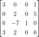
Example 2.2.24. Use GJE to find the inverse of A =  .
.
Solution: Applying GJE to [A|I3] = 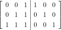 gives
gives
Thus,
A-1 =
.
Definition 2.2.26. [Rank of a Matrix] Let A ∈ Mm,n(ℂ). Then, the rank of A, denoted
Rank(A), is the number of pivots in the RREF(A). For example, Rank(In) = n and Rank(0) = 0.
Remark 2.2.27. Before proceeding further, for A ∈ Mm,n(ℂ), we observe the following.
-
1.
- The number of pivots in the RREF(A) is same as the number of pivots in REF of A.
Hence, we need not compute the RREF(A) to determine the rank of A.
-
2.
- Since, the number of pivots cannot be more than the number of rows or the number of
columns, one has Rank(A) ≤ min{m,n}.
-
3.
- If B =
![[ ]
A 0
0 0](LA444x.png) then Rank(B) = Rank(A) as RREF(B) =
then Rank(B) = Rank(A) as RREF(B) = ![[ ]
RREF (A) 0
0 0](LA445x.png) .
.
-
4.
- If A =
![[ ]
A11 A12
A21 A22](LA446x.png) then, by definition
then, by definition
![([ ]) ([ ])
Rank(A) ≤ Rank A11 A12 + Rank A21 A22 .](LA447x.png) Further, using Remark 2.2.19,
Further, using Remark 2.2.19,
-
(a)
- Rank(A) ≥Rank
![( [ ])
A A
11 12](LA450x.png) .
.
-
(b)
- Rank(A) ≥Rank
![( [ ])
A21 A22](LA451x.png) .
.
-
(c)
- Rank(A) ≥Rank
![( [ ] )
A11
A21](LA452x.png) .
.
We now illustrate the calculation of the rank by giving a few examples.
We now show that the rank doesn’t change if a matrix is multiplied on the left by an invertible
matrix.
Lemma 2.2.29. Let A ∈ Mm,n(ℂ). If S is an invertible matrix then Rank(SA) = Rank(A).

 DRAFT
DRAFT
Proof. By Theorem 2.2.22, RREF(A) = RREF(SA). Hence, Rank(SA) = Rank(A). _
We now have the following result.
Corollary 2.2.30. Let A ∈ Mm,n(ℂ) and B ∈ Mn,q(ℂ). Then, Rank(AB) ≤Rank(A).
In particular, if B ∈ Mn(ℂ) is invertible then Rank(AB) = Rank(A).
Proof. Let Rank(A) = r. Then, there exists an invertible matrix P and A1 ∈ Mr,n(ℂ) such that
PA = RREF(A) = ![[ ]
A1
0](LA459x.png) . Then, PAB =
. Then, PAB = ![[ ]
A1
0](LA460x.png) B =
B = ![[ ]
A1B
0](LA461x.png) . So, using Lemma 2.2.29 and
Remark 2.2.27.2, we get
. So, using Lemma 2.2.29 and
Remark 2.2.27.2, we get
![( [ ] )
A1B
Rank(AB ) = Rank(P AB ) = Rank 0 = Rank (A1B ) ≤ r = Rank(A ).](LA462x.png) | (2.2.4) |
In particular, if B is invertible then, using Equation (2.2.4), we get
 and
hence the required result follows. _
and
hence the required result follows. _
Proof. Let C = RREF(A). Then, by Remark 2.2.19.4 there exists as invertible matrix P such that
C = PA. Note that C has r pivots and they appear in columns, say i1 < i2 <  < ir.
< ir.
Now, let D = CE1i1E2i2 Erir. As Ejij’s are elementary matrices that interchange the columns of
C, one has D =
Erir. As Ejij’s are elementary matrices that interchange the columns of
C, one has D = ![[ ]
Ir B
0 0](LA469x.png) , where B ∈ Mr,n-r(ℂ).
, where B ∈ Mr,n-r(ℂ).
Put Q1 = E1i1E2i2 Erir. Then, Q1 is invertible. Let Q2 =
 ![[ ]
Ir - B
0 In-r](LA471x.png) . Then, verify that Q2 is
invertible and
. Then, verify that Q2 is
invertible and
![[ ] [ ] [ ]
Ir B Ir - B Ir 0
CQ1Q2 = DQ2 = = .
0 0 0 In-r 0 0](LA472x.png) Thus, if we put Q = Q1Q2 then Q is invertible and PAQ = CQ = CQ1Q2 =
Thus, if we put Q = Q1Q2 then Q is invertible and PAQ = CQ = CQ1Q2 = ![[ ]
Ir 0
0 0](LA473x.png) and hence, the
required result follows. _
and hence, the
required result follows. _
We now prove the following result.
Proof. Since A is invertible, RREF(A) = In. Hence, by Remark 2.2.19.4, there exists an invertible
matrix P such that PA = In. Thus,
![[ ]
[ ] [ ] I 0
P A1 P A2 = P A1 A2 = P A = In = r .
0 In-r](LA478x.png) Thus, PA1 =
Thus, PA1 = ![[ ]
Ir
0](LA479x.png) and PA2 =
and PA2 = ![[ ]
0
In-r](LA480x.png) . So, using Corollary 2.2.30, Rank(A1) = r. Also, note that
. So, using Corollary 2.2.30, Rank(A1) = r. Also, note that
![[ ]
0 In- r
Ir 0](LA481x.png) is an invertible matrix and
is an invertible matrix and
![[ ] [ ][ ] [ ]
0 In-r P A = 0 In-r 0 = In-r .
Ir 0 2 Ir 0 In-r 0](LA482x.png) So, again by using Corollary 2.2.30, Rank(A2) = n - r, completing the proof of the first
part.
So, again by using Corollary 2.2.30, Rank(A2) = n - r, completing the proof of the first
part.
For the second part, let us assume that Rank(B1) = t < s. Then, by Remark 2.2.19.4, there exists
an invertible matrix Q such that
for some matrix C, where C is in RREF and has exactly t pivots. Since t < s, QB1 has at least one
zero row.
As PA = In, one has AP = In. Hence, ![[B P ]
1
B2P](LA486x.png) =
= ![[B ]
1
B2](LA487x.png) P = AP = In =
P = AP = In = ![[I 0 ]
s
0 In-s](LA488x.png) .
Thus,
.
Thus,
![[ ] [ ]
B1P = Is 0 and B2P = 0 In-s .](LA489x.png) | (2.2.6) |
Further, using Equations (2.2.5) and (2.2.6), we see that
![[ ] [ ] [ ] [ ]
CP = C P = QB P = Q = .
0 0 1 Is 0 Q 0](LA490x.png) Thus, Q has a zero row, contradicting the assumption that Q is invertible. Hence, Rank(B1) = s.
Similarly, Rank(B2) = n - s and thus, the required result follows. _
Thus, Q has a zero row, contradicting the assumption that Q is invertible. Hence, Rank(B1) = s.
Similarly, Rank(B2) = n - s and thus, the required result follows. _
As a direct corollary of Theorem 2.2.31 and Proposition 2.2.32, we have the following result which
improves Corollary 2.2.30.
Proof. By Theorem 2.2.31, there exist invertible matrices P and Q such that PAQ = ![[ ]
Ir 0
0 0](LA494x.png) . If
P-1 =
. If
P-1 = ![[ ]
B C](LA495x.png) , where B ∈ Mm,r(ℂ) and C ∈ Mm,m-r(ℂ) then,
, where B ∈ Mm,r(ℂ) and C ∈ Mm,m-r(ℂ) then,
![[ ] [ ]
I 0 [ ] I 0 [ ]
AQ = P- 1 r = B C r = B 0 .
0 0 0 0](LA496x.png) Now,
by Proposition 2.2.32, Rank(B) = r = Rank(A) as the matrix P-1 =
Now,
by Proposition 2.2.32, Rank(B) = r = Rank(A) as the matrix P-1 = ![[ ]
B C](LA497x.png) is an invertible matrix.
Thus, the required result follows. _
is an invertible matrix.
Thus, the required result follows. _
As an application of Corollary 2.2.33, we have the following result.
Corollary 2.2.34. Let A ∈ Mm,n(ℂ) and B ∈ Mn,p(ℂ). Then, Rank(AB) ≤Rank(B).
Proof. Let Rank(B) = r. Then, by Corollary 2.2.33, there exists an invertible matrix Q and a matrix
C ∈ Mn,r(ℂ) such that BQ = ![[ ]
C 0](LA498x.png) and Rank(C) = r. Hence, ABQ = A
and Rank(C) = r. Hence, ABQ = A![[ ]
C 0](LA499x.png) =
= ![[ ]
AC 0](LA500x.png) . Thus,
using Corollary 2.2.30 and Remark 2.2.27.2, we get
. Thus,
using Corollary 2.2.30 and Remark 2.2.27.2, we get
![([ ]) |
Rank(AB ) = Rank(ABQ ) = Rank AC 0 = Rank(AC ) ≤ r = Rank(B).](LA501x.png)

 DRAFT
DRAFT
We end this section by relating the rank of the sum of two matrices with sum of their
ranks.
Proposition 2.2.35. Let A,B ∈ Mm,n(ℂ). Then, prove that Rank(A + B) ≤ Rank(A) +
Rank(B). In particular, if A = ∑
i=1kxiyi*, for some xi,yi ∈ ℂ, for 1 ≤ i ≤ k, then
Rank(A) ≤ k.
Proof. Let Rank(A) = r. Then, there exists an invertible matrix P and a matrix A1 ∈ Mr,n(ℂ) such
that PA = RREF(A) = ![[ ]
A1
0](LA504x.png) . Then,
. Then,
![[ ] [ ] [ ]
P (A + B ) = P A + P B = A1 + B1 = A1 + B1 .
0 B2 B2](LA505x.png) Now
using Corollary 2.2.30, Remark 2.2.27.4 and the condition Rank(A) = Rank(A1) = r, the number of
rows of A1, we have
Now
using Corollary 2.2.30, Remark 2.2.27.4 and the condition Rank(A) = Rank(A1) = r, the number of
rows of A1, we have
 Thus, the required result follows. The other part follows, as Rank(xiyi*) = 1, for 1 ≤ i ≤ k. _
Exercise 2.2.36.

 DRAFT
DRAFT
-
1.
- Let A =
![[ ]
2 4 8
1 3 2](LA507x.png) and B =
and B = ![[ ]
1 0 0
0 1 0](LA508x.png) . Find P and Q such that B = PAQ.
. Find P and Q such that B = PAQ.
-
2.
- Let A ∈ Mm,n(ℂ). If Rank(A) = r then, prove that A = BC, where Rank(B) = Rank(C) =
r, B ∈ Mm,r(ℂ) and C ∈ Mr,n(ℂ). Now, use matrix product to give the existence of
xi ∈ ℂm and yi ∈ ℂn such that A = ∑
i=1rxiyi*.
-
3.
- Let A = ∑
i=1kxiyi*, for some xi ∈ ℂm and yi ∈ ℂn. Then does it imply that
Rank(A) ≤ k?
-
4.
- Let
A be a matrix of rank r. Then, prove that there exist invertible matrices Bi,Ci such that
B1A =
![[ ]
R1 R2
0 0](LA511x.png) ,AC1 =
,AC1 = ![[ ]
S1 0
S3 0](LA512x.png) and B2AC2 =
and B2AC2 = ![[ ]
A1 0
0 0](LA513x.png) , where the (1,1) block of
each matrix has size r × r. Also, prove that A1 is an invertible matrix.
, where the (1,1) block of
each matrix has size r × r. Also, prove that A1 is an invertible matrix.
-
5.
- Prove that if Rank(A) = Rank(AB) then A = ABX, for some matrix X. Similarly,
if Rank(A) = Rank(BA) then A = Y BA, for some matrix Y . [Hint: Choose invertible
matrices P,Q satisfying PAQ =
![[ ]
A1 0
0 0](LA514x.png) , P(AB) = (PAQ)(Q-1B) =
, P(AB) = (PAQ)(Q-1B) = ![[ ]
A2 A3
0 0](LA515x.png) . Now,
find an invertible matrix R such that P(AB)R =
. Now,
find an invertible matrix R such that P(AB)R = ![[ ]
C 0
0 0](LA516x.png) . Use the above result to show
that C is invertible. Then X = R
. Use the above result to show
that C is invertible. Then X = R![[ ]
C -1A1 0
0 0](LA517x.png) Q-1 gives the required result.]
Q-1 gives the required result.]
-
6.
- Let P and Q be invertible matrices. Then, prove that Rank(PAQ) = Rank(A).
-
7.
- Let A be an m × n matrix with m ≤ n.
-
(a)
- If P is an invertible matrix such that PA = RREF(A) =
![[ ]
Im 0](LA518x.png) then verify that
P(AAT )PT = (PA)(PA)T = Im and hence prove that Rank(A) = Rank(AAT ).
then verify that
P(AAT )PT = (PA)(PA)T = Im and hence prove that Rank(A) = Rank(AAT ).
-
(b)
- If Q is an invertible matrix such that QAT = RREF(A) =
![[ ]
Im
0](LA519x.png) then verify
that Q(AT A)QT = (QAT )(QAT )T =
then verify
that Q(AT A)QT = (QAT )(QAT )T = ![[I 0]
m
0 0](LA520x.png) and hence prove that Rank(A) =
Rank(AT A).
and hence prove that Rank(A) =
Rank(AT A).
-
(c)
- Generalize the above ideas to prove that if Rank(A) = m then Rank(A) =
Rank(AT A) = Rank(AAT ).

 DRAFT
DRAFT
Definition 2.2.37. [Basic, Free Variables] Consider the linear system Ax = b. If
RREF([Ab]) = [Cd]. Then, the variables corresponding to the pivotal columns of C are called
the basic variables and the variables that are not basic are called free variables.
We now prove the main result in the theory of linear systems. Before doing so, we look at the following
example.
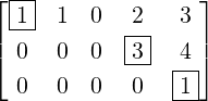
Example 2.2.39. Consider a linear system Ax = b. Suppose RREF([Ab]) = [Cd], where
![⌊|-| ⌋
|-1- |0| 2 - 1 0 0 2 8|
|| 0 -1- 1 3 |0| 0 5 1||
|| 0 0 0 0 |1| 0 - 1 2||
[Cd ] = | --- |-| | .
|| 0 0 0 0 0 -1- 1 4||
|⌈ 0 0 0 0 0 0 0 0|⌉
0 0 0 0 0 0 0 0](LA528x.png)
Then
to get the solution set, we observe the following.
-
1.
- C has 4 pivotal columns, namely, the columns 1,2,5 and 6. Thus, x1,x2,x5 and x6 are
basic variables.
-
2.
- Hence, the remaining variables, x3,x4 and x7 are free variables.
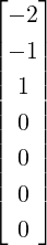
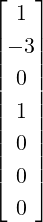
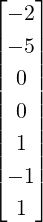
Therefore, the solution set is given by

 DRAFT
DRAFT
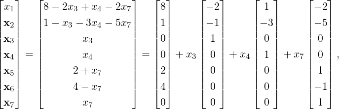
where
x3,x4 and
x7 are arbitrary.
Let
x0 =
 ,u1
,u1 =
 ,u2
,u2 =
and
u3 =
. In this example, verify that
Cx0 =
d, and for 1
≤ i ≤ 3,
Cui =
0. Hence, it follows that
Ax0 =
d, and for 1
≤ i ≤ 3,
Aui =
0.
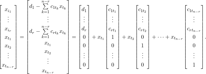
Theorem 2.2.40. Let Ax = b be a linear system in n variables with RREF([Ab]) = [Cd] with
Rank(A) = r and Rank([Ab]) = ra.
-
1.
- Then, the system Ax = b is inconsistent if r < ra
-
2.
- Then, the system Ax = b is consistent if r = ra.
-
(a)
- Further, Ax = b has a unique solution if r = n.
-
(b)
- Further, Ax = b has infinite number of solutions if r < n. In this case, there
exist vectors x0,u1,…,un-r ∈ ℝn with Ax0 = b and Aui = 0, for 1 ≤ i ≤ n - r.
Furthermore, the solution set is given by

 DRAFT
DRAFT

Proof. Part 1: As r < ra, by Remark 2.2.19.5 ([Cd])[r + 1,:] = [0T 1]. Note that this row corresponds
to the linear equation
 which clearly has no solution. Thus, by definition and Theorem 2.1.17, Ax = b is inconsistent.
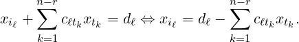
Part 2: As r = ra, by Remark 2.2.19.5, [Cd] doesn’t have a row of the form [0T 1]. Further, the
number of pivots in [Cd] and that in C is same, namely, r pivots. Suppose the pivots appear in
columns i1,…,ir with 1 ≤ i1 <  < ir ≤ n. Thus, the variables xij, for 1 ≤ j ≤ r, are basic variables
and the remaining n-r variables, say xt1,…,xtn-r, are free variables with t1 <
< ir ≤ n. Thus, the variables xij, for 1 ≤ j ≤ r, are basic variables
and the remaining n-r variables, say xt1,…,xtn-r, are free variables with t1 <  < tn-r. Since C is
in RREF, in terms of the free variables and basic variables, the ℓ-th row of [Cd], for 1 ≤ ℓ ≤ r,
corresponds to the equation
< tn-r. Since C is
in RREF, in terms of the free variables and basic variables, the ℓ-th row of [Cd], for 1 ≤ ℓ ≤ r,
corresponds to the equation
 Thus, the system Cx = d is consistent. Hence, by Theorem 2.1.17 the system Ax = b is consistent
and the solution set of the system Ax = b and Cx = d are the same. Therefore, the solution set of the
system Cx = d (or equivalently Ax = b) is given by
Thus, the system Cx = d is consistent. Hence, by Theorem 2.1.17 the system Ax = b is consistent
and the solution set of the system Ax = b and Cx = d are the same. Therefore, the solution set of the
system Cx = d (or equivalently Ax = b) is given by
Part 2a: As r = n, there are no free variables. Hence, xi = di, for 1 ≤ i ≤ n, is the unique
solution.
Part 2b: Define x0 = 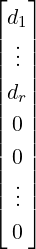 and u1 =
 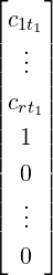 ,…,un-r =
 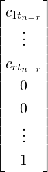 . Then, it can be easily verified
that Ax0 = b and, for 1 ≤ i ≤ n - r, Aui = 0. Also, by Equation (2.2.7) the solution set has indeed
the required form, where ki corresponds to the free variable xti. As there is at least one free
variable the system has infinite number of solutions. Thus, the proof of the theorem is
complete. _
. Then, it can be easily verified
that Ax0 = b and, for 1 ≤ i ≤ n - r, Aui = 0. Also, by Equation (2.2.7) the solution set has indeed
the required form, where ki corresponds to the free variable xti. As there is at least one free
variable the system has infinite number of solutions. Thus, the proof of the theorem is
complete. _
Let A ∈ Mm,n(ℂ). Then, Rank(A) ≤ m. Thus, using Theorem 2.2.40 the next result
follows.
Corollary 2.2.42. Let A ∈ Mm,n(ℂ). If Rank(A) = r < min{m,n} then Ax = 0 has infinitely
many solutions. In particular, if m < n, then Ax = 0 has infinitely many solutions. Hence, in
either case, the homogeneous system Ax = 0 has at least one non-trivial solution.
Remark 2.2.43. Let A ∈ Mm,n(ℂ). Then, Theorem 2.2.40 implies that Ax = b is consistent
if and only if Rank(A) = Rank([Ab]). Further, the vectors associated to the free variables in
Equation (2.2.7) are solutions to the associated homogeneous system Ax = 0.
We end this subsection with some applications.
Example 2.2.44.
-
1.
- Determine the equation of the line/circle that passes through the points (-1,4),(0,1)
and (1,4).
Solution: The general equation of a line/circle in Euclidean plane is given by a(x2 +
y2) + bx + cy + d = 0, where a,b,c and d are variables. Since this curve passes
through the given points, we get a homogeneous system in 3 equations and 4 variables,

 DRAFT
namely
DRAFT
namely 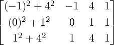
 = 0. Solving this system, we get [a,b,c,d] =
[
= 0. Solving this system, we get [a,b,c,d] =
[ d,0,-
d,0,- d,d]. Hence, choosing d = 13, the required circle is given by 3(x2 +y2)-16y +
13 = 0.
d,d]. Hence, choosing d = 13, the required circle is given by 3(x2 +y2)-16y +
13 = 0.
-
2.
- Determine the equation of the plane that contains the points (1,1,1),(1,3,2) and
(2,-1,2).
Solution: The general equation of a plane in space is given by ax + by + cz + d = 0,
where a,b,c and d are variables. Since this plane passes through the 3 given points, we
get a homogeneous system in 3 equations and 4 variables. So, it has a non-trivial solution,
namely [a,b,c,d] = [- d,-
d,- ,-
,- d,d]. Hence, choosing d = 3, the required plane is given
by -4x - y + 2z + 3 = 0.
d,d]. Hence, choosing d = 3, the required plane is given
by -4x - y + 2z + 3 = 0.
-
3.
- Let A =
 . Then, find a non-trivial solution of Ax = 2x. Does there exist a
nonzero vector y ∈ ℝ3 such that Ay = 4y?
. Then, find a non-trivial solution of Ax = 2x. Does there exist a
nonzero vector y ∈ ℝ3 such that Ay = 4y?
Solution: Solving for Ax = 2x is equivalent to solving (A - 2I)x = 0. The augmented
matrix of this system equals  . Verify that xT
= [1,0,0] is a nonzero
solution. For the other part, the augmented matrix for solving (A - 4I)y = 0 equals
. Verify that xT
= [1,0,0] is a nonzero
solution. For the other part, the augmented matrix for solving (A - 4I)y = 0 equals
 . Thus, verify that yT
= [2,0,1] is a nonzero solution.
. Thus, verify that yT
= [2,0,1] is a nonzero solution.
Exercise 2.2.45.
-
1.
- Let A ∈ Mn(ℂ). If A2x = 0 has a non trivial solution then show that Ax = 0 also has a
non trivial solution.
-
2.
- Prove that 5 distinct points are needed to specify a general conic, namely, ax2 + by2 +
cxy + dx + ey + f = 0, in the Euclidean plane.

 DRAFT
DRAFT
-
3.
- Let u = (1,1,-2)T and v = (-1,2,3)T . Find condition on x,y and z such that the system
cu + dv = (x,y,z)T in the variables c and d is consistent.
-
4.
- For what values of c and k, the following systems have i) no solution, ii) a unique solution and
iii) infinite number of solutions.
-
(a)
- x + y + z = 3,x + 2y + cz = 4,2x + 3y + 2cz = k.
-
(b)
- x + y + z = 3,x + y + 2cz = 7,x + 2y + 3cz = k.
-
(c)
- x + y + 2z = 3,x + 2y + cz = 5,x + 2y + 4z = k.
-
5.
- Find the condition(s) on x,y,z so that the systems given below (in the variables a,b and c) is
consistent?
-
(a)
- a + 2b - 3c = x,2a + 6b - 11c = y,a - 2b + 7c = z.
-
(b)
- a + b + 5c = x,a + 3c = y,2a - b + 4c = z.
_____________________________________
-
6.
- Determine the equation of the curve y = ax2 + bx + c that passes through the points
(-1,4),(0,1) and (1,4).
-
7.
- Solve the linear systems
x + y + z + w = 0,x - y + z + w = 0 and -x + y + 3z + 3w = 0, and
x + y + z = 3,x + y - z = 1,x + y + 4z = 6 and x + y - 4z = -1.
-
8.
- For what values of a, does the following systems have i) no solution, ii) a unique solution and
iii) infinite number of solutions.
-
(a)
- x + 2y + 3z = 4,2x + 5y + 5z = 6,2x + (a2 - 6)z = a + 20.
-
(b)
- x + y + z = 3,2x + 5y + 4z = a,3x + (a2 - 8)z = 12.
-
9.
- Consider the linear system Ax = b in m equations and 3 variables. Then, for each of the given
solution set, determine the possible choices of m? Further, for each choice of m, determine a
choice of A and b.

 DRAFT
DRAFT
-
(a)
- (1,1,1)T is the only solution.
-
(b)
- {(1,1,1)T + c(1,2,1)T |c ∈ ℝ} as the solution set.
-
(c)
- {c(1,2,1)T |c ∈ ℝ} as the solution set.
-
(d)
- {(1,1,1)T + c(1,2,1)T + d(2,2,-1)T |c,d ∈ ℝ} as the solution set.
-
(e)
- {c(1,2,1)T + d(2,2,-1)T |c,d ∈ ℝ} as the solution set.
In this section the coefficient matrix of the linear system Ax = b will be a square matrix. We start
with proving a few equivalent conditions that relate different ideas.
Theorem 2.3.1. Let A ∈ Mn(ℂ). Then, the following statements are equivalent.
-
1.
- A is invertible.
-
2.
- RREF(A) = In.
-
3.
- A is a product of elementary matrices.
-
4.
- The homogeneous system Ax = 0 has only the trivial solution.
-
5.
- Rank(A) = n.
Proof. 1 ⇔2 Already done in Proposition 2.2.21.
2 ⇔3 Again, done in Proposition 2.2.21.

 DRAFT
DRAFT
3  4 Let A = E1
 Ek, for some elementary matrices E1,…,Ek. Then, by previous
equivalence A is invertible. So, A-1 exists and A-1A = In. Hence, if x0 is any solution of the
homogeneous system Ax = 0 then,
Ek, for some elementary matrices E1,…,Ek. Then, by previous
equivalence A is invertible. So, A-1 exists and A-1A = In. Hence, if x0 is any solution of the
homogeneous system Ax = 0 then,
 Thus, 0 is the only solution of the homogeneous system Ax = 0.
4  5 Let if possible Rank(A) = r < n. Then, by Corollary 2.2.42, the homogeneous
system Ax = 0 has infinitely many solution. A contradiction. Thus, A has full rank.
5 Let if possible Rank(A) = r < n. Then, by Corollary 2.2.42, the homogeneous
system Ax = 0 has infinitely many solution. A contradiction. Thus, A has full rank.
5  2 Suppose Rank(A) = n. So, RREF(A) has n pivotal columns. But, RREF(A) has
exactly n columns and hence each column is a pivotal column. Thus, RREF(A) = In. _
2 Suppose Rank(A) = n. So, RREF(A) has n pivotal columns. But, RREF(A) has
exactly n columns and hence each column is a pivotal column. Thus, RREF(A) = In. _
We end this section by giving two more equivalent conditions for a matrix to be invertible.
Theorem 2.3.2. The following statements are equivalent for A ∈ Mn(ℂ).
-
1.
- A is invertible.
-
2.
- The system Ax = b has a unique solution for every b.
-
3.
- The system Ax = b is consistent for every b.
Proof. 1  2 Note that x0 = A-1b is the unique solution of Ax = b.
2  3 The system is consistent as Ax = b has a solution.
3  1 For 1 ≤ i ≤ n, define eiT = In[i,:]. By assumption, the linear system Ax = ei has a
solution, say xi, for 1 ≤ i ≤ n. Define a matrix B = [x1,…,xn]. Then,
1 For 1 ≤ i ≤ n, define eiT = In[i,:]. By assumption, the linear system Ax = ei has a
solution, say xi, for 1 ≤ i ≤ n. Define a matrix B = [x1,…,xn]. Then,

 DRAFT
DRAFT
![AB = A [x1,x2...,xn] = [Ax1, Ax2 ...,Axn ] = [e1,e2 ...,en ] = In.](LA578x.png) Therefore, n = Rank(In) = Rank(AB) ≤Rank(A) and hence Rank(A) = n. Thus, by Theorem 2.3.1, A
is invertible. _
Therefore, n = Rank(In) = Rank(AB) ≤Rank(A) and hence Rank(A) = n. Thus, by Theorem 2.3.1, A
is invertible. _
We now give an immediate application of Theorem 2.3.2 and Theorem 2.3.1 without
proof.
Theorem 2.3.3. The following two statements cannot hold together for A ∈ Mn(ℂ).
-
1.
- The system Ax = b has a unique solution for every b.
-
2.
- The system Ax = 0 has a non-trivial solution.
As an immediate consequence of Theorem 2.3.1, the readers should prove that one needs to
compute either the left or the right inverse to prove invertibility of A ∈ Mn(ℂ).
Corollary 2.3.4. Let A ∈ Mn(ℂ). Then, the following holds.
-
1.
- Suppose there exists C such that CA = In. Then, A-1 exists.
-
2.
- Suppose there exists B such that AB = In. Then, A-1 exists.
Exercise 2.3.5.
-
1.
- Let A be a square matrix. Then, prove that A is invertible ⇔ AT is invertible ⇔ AT A is
invertible ⇔ AAT is invertible.

 DRAFT
DRAFT
-
2.
- [Theorem of the Alternative] The following two statements cannot hold together for
A ∈ Mn(ℂ) and b ∈ ℝn.
-
(a)
- The system Ax = b has a solution.
-
(b)
- The system yT A = 0T ,yT b≠0 has a solution.
__________________________________
-
3.
- Let A and B be two matrices having positive entries and of orders 1 ×n and n× 1, respectively.
Which of BA or AB is invertible? Give reasons.
-
4.
- Let A ∈ Mn,m(ℂ) and B ∈ Mn,m(ℂ).
-
(a)
- Then, prove that I - BA is invertible if and only if I - AB is invertible [use
Theorem 2.3.1.4].
-
(b)
- If I - AB is invertible then, prove that (I - BA)-1 = I + B(I - AB)-1A.
-
(c)
- If I - AB is invertible then, prove that (I - BA)-1B = B(I - AB)-1.
-
(d)
- If A,B and A + B are invertible then, prove that (A-1 + B-1)-1 = A(A + B)-1B.
-
5.
- Let bT = [1,2,-1,-2]. Suppose A is a 4 × 4 matrix such that the linear system Ax = b has no
solution. Mark each of the statements given below as true or false?
-
(a)
- The homogeneous system Ax = 0 has only the trivial solution.
-
(b)
- The matrix A is invertible.
-
(c)
- Let cT = [-1,-2,1,2]. Then, the system Ax = c has no solution.
-
(d)
- Let B = RREF(A). Then,
-
i.
- B[4,:] = [0,0,0,0].
-
ii.
- B[4,:] = [0,0,0,1].
-
iii.
- B[3,:] = [0,0,0,0].

 DRAFT
DRAFT
-
iv.
- B[3,:] = [0,0,0,1].
-
v.
- B[3,:] = [0,0,1,α], where α is any real number.
In this section, we associate a number with each square matrix. To start with, recall the notations
used in Section 1.3.1. Then, for A =  , A(1|2) =
 ![[ ]
1 2
2 7](LA586x.png) and A({1,2}|{1,3}) = [4].
and A({1,2}|{1,3}) = [4].
With the notations as above, we are ready to give an inductive definition of the determinant of a
square matrix. The advanced students can find an alternate definition of the determinant in
Appendix 9.2.22, where it is proved that the definition given below corresponds to the expansion of
determinant along the first row.
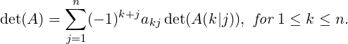
Definition 2.3.6. Let A be a square matrix of order n. Then, the determinant of A, denoted
det(A) (or |A|) is defined by
,
det(A ) = n∑ 1+j
|( (- 1) a1j det(A (1|j)), otherwise.
j=1](LA587x.png)

 DRAFT
Definition 2.3.9. [Singular, Non-Singular Matrices] A matrix A is said to be a singular
if det(A) = 0 and is called non-singular if det(A)≠0.
DRAFT
Definition 2.3.9. [Singular, Non-Singular Matrices] A matrix A is said to be a singular
if det(A) = 0 and is called non-singular if det(A)≠0.
The next result relates the determinant with row operations. For proof, see Appendix 9.3.
Theorem 2.3.10. Let A be an n × n matrix.
-
1.
- If B = EijA, for 1 ≤ i≠j ≤ n, then det(B) = -det(A).
-
2.
- If B = Ei(c)A, for c≠0,1 ≤ i ≤ n, then det(B) = cdet(A).
-
3.
- If B = Eij(c)A, for c≠0 and 1 ≤ i≠j ≤ n, then det(B) = det(A).
-
4.
- If A[i,:]T = 0, for 1 ≤ i,j ≤ n then det(A) = 0.
-
5.
- If A[i,:] = A[j,:] for 1 ≤ i≠j ≤ n then det(A) = 0.
-
6.
- If A is a triangular matrix with d1,…,dn on the diagonal then det(A) = d1
 dn.
dn.
As det(In) = 1, we have the following result.
Corollary 2.3.11. Fix a positive integer n.
-
1.
- Then, det(Eij) = -1.
-
2.
- If c≠0 then, det(Ek(c)) = c.
-
3.
- If c≠0 then, det(Eij(c)) = 1.

 DRAFT
DRAFT
By Theorem 2.3.10.6 det(In) = 1. The next result about the determinant of elementary matrices is
an immediate consequence of Theorem 2.3.10 and hence the proof is omitted.
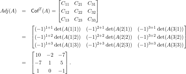
Definition 2.3.16. Let A ∈ Mn(ℂ). Then, the cofactor matrix, denoted Cof(A), is an
Mn(ℂ) matrix with Cof(A) = [Cij], where

And, the
Adjugate (classical Adjoint) of
A, denoted
Adj(
A), equals
CofT (
A).

 DRAFT
DRAFT
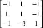
Example 2.3.17. Let A =  .
.
-
1.
- Then, Now, verify that AAdj(A) =
 =
=  = Adj(A)A.
-
2.
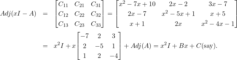
- Consider xI3 - A =
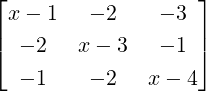 . Then, Hence, we observe that Adj(xI - A) = x2I + Bx + C is a polynomial in x with coefficients as
matrices. Also, note that (xI - A)Adj(xI - A) = (x3 - 8x2 + 10x - det(A))I3. Thus, we see
that
. Then, Hence, we observe that Adj(xI - A) = x2I + Bx + C is a polynomial in x with coefficients as
matrices. Also, note that (xI - A)Adj(xI - A) = (x3 - 8x2 + 10x - det(A))I3. Thus, we see
that
 That is, we have obtained a matrix equality and hence, replacing x by A makes sense. But, then
the LHS is 0. So, for the RHS to be zero, we must have A3 - 8A2 + 10A - det(A)I = 0 (this
equality is famously known as the Cayley-Hamilton Theorem).
That is, we have obtained a matrix equality and hence, replacing x by A makes sense. But, then
the LHS is 0. So, for the RHS to be zero, we must have A3 - 8A2 + 10A - det(A)I = 0 (this
equality is famously known as the Cayley-Hamilton Theorem).
The next result relates adjugate matrix with the inverse, in case det(A)≠0.
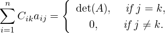
Theorem 2.3.18. Let A ∈ Mn(ℂ).
-
1.
- Then, ∑
j=1naijCij = ∑
j=1naij(-1)i+j det(A(i|j)) = det(A), for 1 ≤ i ≤ n.
-
2.
- Then, ∑
j=1naijCℓj = ∑
j=1naij(-1)i+j det(A(ℓ|j)) = 0, for i≠ℓ.
-
3.
- Thus, A(Adj(A)) = det(A)In. Hence,
Proof. Part 1: It follows directly from Remark 2.3.14 and the definition of the cofactor.
Part 2: Fix positive integers i,ℓ with 1 ≤ i≠ℓ ≤ n and let B = [bij] be a square matrix with
B[ℓ,:] = A[i,:] and B[t,:] = A[t,:], for t≠ℓ. As ℓ≠i, B[ℓ,:] = B[i,:] and thus, by Theorem 2.3.10.5,
det(B) = 0. As A(ℓ|j) = B(ℓ|j), for 1 ≤ j ≤ n, using Remark 2.3.14
This completes the proof of Part 2.
Part 3: Using Equation (2.3.2) and Remark 2.3.14, observe that
![{
∑n ∑n 0, if i ⁄= j,
[A(Adj (A ))]ij = aik(Adj(A ))kj = aikCjk = det(A ), if i = j.
k=1 k=1
<img
src=](LA639x.png)
 DRAFT
" class="math-display" >
DRAFT
" class="math-display" >
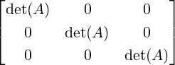
Thus, A(Adj(A)) = det(A)In. Therefore, if det(A)≠0 then A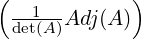 = In. Hence, by
Proposition 2.2.21, A-1 =
= In. Hence, by
Proposition 2.2.21, A-1 =  Adj(A). _
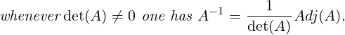
Let A be a non-singular matrix. Then, by Theorem 2.3.18.3, A-1 =  Adj(A). Thus
A
Adj(A). Thus
A Adj(A)
 =
=  Adj(A)
 A = det(A)In and this completes the proof of the next result
Corollary 2.3.20. Let A be a non-singular matrix. Then,
The next result gives another equivalent condition for a square matrix to be invertible.
Theorem 2.3.21. A square matrix A is non-singular if and only if A is invertible.

 DRAFT
DRAFT
Proof. Let A be non-singular. Then, det(A)≠0 and hence A-1 =  Adj(A).
Now, let us assume that A is invertible. Then, using Theorem 2.3.1, A = E1 Ek, a product of
elementary matrices. Also, by Corollary 2.3.11, det(Ei)≠0, for 1 ≤ i ≤ k. Thus, a repeated application
of Parts 1,2 and 3 of Theorem 2.3.10 gives det(A)≠0. _
Ek, a product of
elementary matrices. Also, by Corollary 2.3.11, det(Ei)≠0, for 1 ≤ i ≤ k. Thus, a repeated application
of Parts 1,2 and 3 of Theorem 2.3.10 gives det(A)≠0. _
The next result relates the determinant of a matrix with the determinant of its transpose. Thus,
the determinant can be computed by expanding along any column as well.
Theorem 2.3.22. Let A be a square matrix. Then, det(A) = det(AT ).
Proof. If A is a non-singular, Corollary 2.3.20 gives det(A) = det(AT ).
If A is singular then, by Theorem 2.3.21, A is not invertible. So, AT is also not invertible and
hence by Theorem 2.3.21, det(AT ) = 0 = det(A). _
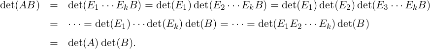
The next result relates the determinant of product of two matrices with their determinants.
Theorem 2.3.23. Let A and B be square matrices of order n. Then,

Proof. Case 1: Let A be non-singular. Then, by Theorem 2.3.18.3, A is invertible and by
Theorem 2.3.1, A = E1 Ek, a product of elementary matrices. Thus, a repeated application of Parts
1,2 and 3 of Theorem 2.3.10 gives the desired result as
Ek, a product of elementary matrices. Thus, a repeated application of Parts
1,2 and 3 of Theorem 2.3.10 gives the desired result as
Case 2: Let A be singular. Then, by Theorem 2.3.21 A is not invertible. So, by Proposition 2.2.21
there exists an invertible matrix P such that PA = ![[ ]
C1
0](LA662x.png) . So, A = P-1
. So, A = P-1![[ ]
C1
0](LA663x.png) . As P is invertible,
using Part 1, we have
. As P is invertible,
using Part 1, we have
Thus, the proof of the theorem is complete. _
Example 2.3.24. Let A be an orthogonal matrix then, by definition, AAT = I. Thus, by
Theorems 2.3.23 and 2.3.22

Hence det
A =
±1. In particular, if
A =
![[ ]
a b
c d](LA666x.png)
then
I =
AAT =
![[ ]
a2 + b2 ac+ bd
ac + bd c2 + d2](LA667x.png)
.

 DRAFT
DRAFT
-
1.
- Thus, a2 + b2 = 1 and hence there exists θ ∈ [-pi,π) such that a = cosθ and b = sinθ.
-
2.
- As ac + bd = 0, we get c = r sinθ and d = -r cosθ, for some r ∈ ℝ. But, c2 + d2 = 1
implies that either c = sinθ and d = -cosθ or c = -sinθ and d = cosθ.
-
3.
- Thus, A =
![[ ]
cosθ sinθ
sinθ - cosθ](LA670x.png) or A =
or A = ![[ ]
cosθ sin θ
- sin θ cosθ](LA671x.png) .
.
-
4.
- For A =
![[ ]
cosθ sin θ
sin θ - cosθ](LA672x.png) , det(A) = -1. Then A represents a reflection across the line
y = mx. Determine m? (see Exercise 2.2b).
, det(A) = -1. Then A represents a reflection across the line
y = mx. Determine m? (see Exercise 2.2b).
-
5.
- For A =
![[ cosθ sin θ]
- sin θ cosθ](LA673x.png) , det(A) = 1. Then A represents a rotation through the angle α.
Determine α? (see Exercise 2.2a).
, det(A) = 1. Then A represents a rotation through the angle α.
Determine α? (see Exercise 2.2a).
Exercise 2.3.25.
-
1.
- Let A ∈ Mn(ℂ) be an upper triangular matrix with nonzero entries on the diagonal. Then,
prove that A-1 is also an upper triangular matrix.___________________________________
-
2.
- Let A ∈ Mn(ℂ). Then, det(A) = 0 if
-
(a)
- either A[i,:]T = 0T or A[:,i] = 0, for some i,1 ≤ i ≤ n,
-
(b)
- or A[i,:] = cA[j,:], for some c ∈ ℂ and for some i≠j,
-
(c)
- or A[:,i] = cA[:,j], for some c ∈ ℂ and for some i≠j,
-
(d)
- or A[i,:] = c1A[j1,:] + c2A[j2,:] +
 + ckA[jk,:], for some rows i,j1,…,jk of A and
some ci’s in ℂ,
+ ckA[jk,:], for some rows i,j1,…,jk of A and
some ci’s in ℂ,
-
(e)
- or A[:,i] = c1A[:,j1] + c2A[:,j2] +
 + ckA[:,jk], for some columns i,j1,…,jk of A
and some ci’s in ℂ.
+ ckA[:,jk], for some columns i,j1,…,jk of A
and some ci’s in ℂ.
-

 DRAFT
3.
DRAFT
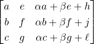
3. - Let A =
 and B =
 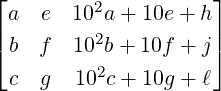 , where a,b…,ℓ ∈ ℂ. Without computing
deduce that det(A) = det(B). Hence, conclude that 17 divides
, where a,b…,ℓ ∈ ℂ. Without computing
deduce that det(A) = det(B). Hence, conclude that 17 divides  .
.
Let A be a square matrix. Then, combining Theorem 2.3.2 and Theorem 2.3.21, one has the following
result.
Corollary 2.3.26. Let A be a square matrix. Then, the following statements are equivalent:
-
1.
- A is invertible.
-
2.
- The linear system Ax = b has a unique solution for every b.
-
3.
- det(A)≠0.
Thus, Ax = b has a unique solution for every b if and only if det(A)≠0. The next
theorem gives a direct method of finding the solution of the linear system Ax = b when
det(A)≠0.
Theorem 2.3.27 (Cramer’s Rule). Let A be an n × n non-singular matrix. Then, the unique
solution of the linear system Ax = b with xT = [x1,…,xn] is given by

 DRAFT
DRAFT
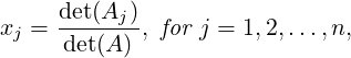 where Aj is the matrix obtained from A by replacing A
[:
,j]
by b.
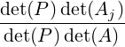
Proof. Since det(A)≠0, A is invertible. Thus, there exists an invertible matrix P such that PA = In
and P[A|b] = [I|Pb]. Then A-1 = P. Let d = Pb = A-1b. Then, Ax = b has the unique
solution xj = dj, for 1 ≤ j ≤ n. Also, [e1,…,en] = I = PA = [PA[:,1],…,PA[:,n]]. Thus,
Thus, det(PAj) = dj, for 1 ≤ j ≤ n. Also, dj =  =
=  =
=  =
=  . Hence,
xj =
. Hence,
xj =  and the required result follows. _
Exercise 2.4.1.
-
1.
- Let A be a unitary matrix then what can you say about ∣det(A)∣?
-
2.
- Let A ∈ Mn(ℂ). Prove that the following statements are equivalent:
-
(a)
- A is not invertible.
-
(b)
- Rank(A)≠n.
-
(c)
- det(A) = 0.
-
(d)
- A is not row-equivalent to In.
-
(e)
- The homogeneous system Ax = 0 has a non-trivial solution.
-
(f)
- The system Ax = b is either inconsistent or it has an infinite number of solutions.
-
(g)
- A is not a product of elementary matrices.
-
3.
- Let A be a Hermitian matrix. Prove that detA is a real number.
-
4.
- Let A ∈ Mn(ℂ). Then, A is invertible if and only if Adj(A) is invertible.

 DRAFT
DRAFT
-
5.
- Let A and B be invertible matrices. Prove that Adj(AB) = Adj(B)Adj(A).
-
6.
- Let A be an invertible matrix and let P =
![[ ]
A B
C D](LA697x.png) . Then, show that Rank(P) = n if and only if
D = CA-1B._____________________________________________________________________
. Then, show that Rank(P) = n if and only if
D = CA-1B._____________________________________________________________________ -
7.
- Let A be a 2 × 2 matrix with tr(A) = 0 and det(A) = 0. Then, A is a nilpotent
matrix.
-
8.
- Determine necessary and sufficient condition for a triangular matrix to be invertible.
-
9.
- Suppose A-1 = B with A =
![[ ]
A11 A12
A21 A22](LA698x.png) and B =
and B = ![[ ]
B11 B12
B21 B22](LA699x.png) . Also, assume that A11 is
invertible and define P = A22 - A21A11-1A12. Then, prove that
. Also, assume that A11 is
invertible and define P = A22 - A21A11-1A12. Then, prove that
-
(a)
-
![[ ]
I 0
-1
- A21A 11 I](LA700x.png)
![[ ]
A11 A12
A21 A22](LA701x.png) =
= ![[ ]
A11 A12
-1
0 A22 - A21A 11 A12](LA702x.png) ,
,
-
(b)
- P is invertible and B =
![[ -1 - 1 -1 -1 -1 -1]
A11 + (A11 A12 )P (A21A 11 ) - (A 11 A12)P
- P -1(A21A -111 ) P -1](LA703x.png) .
.
-
10.
- Let A and B be two non-singular matrices. Are the matrices A + B and A - B non-singular?
Justify your answer.
-
11.
- For what value(s) of λ does the following systems have non-trivial solutions? Also, for each
value of λ, determine a non-trivial solution.
-
(a)
- (λ - 2)x + y = 0,x + (λ + 2)y = 0.
-
(b)
- λx + 3y = 0,(λ + 6)y = 0.
-
12.
- Let a1,…,an ∈ ℂ and define A = [aij]n×n with aij = aij-1. Prove that det(A) = ∏
1≤i<j≤n(aj -ai).
This matrix is usually called the van der monde matrix.
-
13.
- Let A = [aij] ∈ Mn(ℂ) with aij = max{i,j}. Prove that detA = (-1)n-1n.
-
14.
- Solve the following linear system by Cramer’s rule.
i)x + y + z - w = 1,x + y - z + w = 2, 2x + y + z - w = 7,x + y + z + w = 3.
ii)x - y + z - w = 1,x + y - z + w = 2, 2x + y - z - w = 7,x - y - z + w = 3.

 DRAFT
DRAFT
-
15.
- Let p ∈ ℂ,p≠0. Let A = [aij],B = [bij] ∈ Mn(ℂ) with bij = pi-jaij, for 1 ≤ i,j ≤ n. Then,
compute det(B) in terms of det(A).
-
16.
- The position of an element aij of a determinant is called even or odd according as i + j is even
or odd. Prove that if all the entries in
-
(a)
- odd positions are multiplied with -1 then the value of determinant doesn’t change.
-
(b)
- even positions are multiplied with -1 then the value of determinant
-
i.
- does not change if the matrix is of even order.
-
ii.
- is multiplied by -1 if the matrix is of odd order.
In this chapter, we started with a system of m linear equations in n variables and formally wrote it as
Ax = b and in turn to the augmented matrix [A|b]. Then, the basic operations on equations led to
multiplication by elementary matrices on the right of [A|b]. These elementary matrices are
invertible and applying the GJE on a matrix A, resulted in getting the RREF of A. We
used the pivots in RREF matrix to define the rank of a matrix. So, if Rank(A) = r and
Rank([A|b]) = ra
-
1.
- then, r < ra implied the linear system Ax = b is inconsistent.
-
2.
- then, r = ra implied the linear system Ax = b is consistent. Further,
-
(a)
- if r = n then the system Ax = b has a unique solution.
-
(b)
- if r < n then the system Ax = b has an infinite number of solutions.
We have also seen that the following conditions are equivalent for A ∈ Mn(ℂ).

 DRAFT
DRAFT
-
1.
- A is invertible.
-
2.
- The homogeneous system Ax = 0 has only the trivial solution.
-
3.
- The row reduced echelon form of A is I.
-
4.
- A is a product of elementary matrices.
-
5.
- The system Ax = b has a unique solution for every b.
-
6.
- The system Ax = b has a solution for every b.
-
7.
- Rank(A) = n.
-
8.
- det(A)≠0.
So, overall we have learnt to solve the following type of problems:
-
1.
- Solving the linear system Ax = b. This idea will lead to the question “is the vector b a
linear combination of the columns of A”?
-
2.
- Solving the linear system Ax = 0. This will lead to the question “are the columns of A linearly
independent/dependent”? In particular, we will see that
-
(a)
- if Ax = 0 has a unique solution then the columns of A are linear independent.
-
(b)
- if Ax = 0 has a non-trivial solution then the columns of A are linearly dependent.

 DRAFT
DRAFT

 DRAFT
DRAFT

 DRAFT
DRAFT


 ,
,
 and
and  . Then, (
![[Ab ]](LA287x.png) is called the
is called the  and
and  equals
  .
.


 ,
,  ,
,  and
and  .
.


 . Then, verify that
 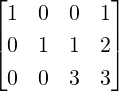 .
.

![[ ]
2 1
1 2](LA333x.png) =
= 
 =
= 

 and
and  row equivalent?
  is a solution of

 ,
,  ,
,  and
and  .
.
 and
and 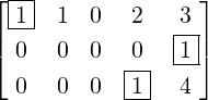 .
. ,
,  ,
,  and
and 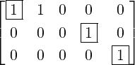 .
.


 ,
,  ,
,  .
.


![[ ]
A B](LA422x.png)
![[ ]
A
B](LA423x.png)
![[ ]
In A-1B](LA424x.png)
![[ ]
In
0](LA425x.png)
![⌊ | ⌋ ⌊ | ⌋
E |1 1 1 |0 0 1| E13(-1),E23(-2)|1 1 0 |- 1 0 1|
[A|I3] 1→3 ⌈0 1 1 |0 1 0⌉ → ⌈0 1 0 |- 1 1 0⌉
0 0 1 |1 0 0 0 0 1 | 1 0 0
⌊ | ⌋
1 0 0 | 0 - 1 1
E12(→-1) |⌈0 1 0 |- 1 1 0|⌉.
|
0 0 1 | 1 0 0](LA436x.png)


 (
( (
( (
(
![[ ]
1 1
2 2](LA453x.png) and
and ![[ ]
- 1 1
1 - 1](LA454x.png) . Then,
. Then, ![[ ]
1 1
- 1 - 1](LA455x.png) . So,
. So, 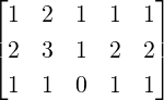 . Then,

![[ ]
P AQ = Ir 0 .
0 0](LA466x.png)


![[ ]
A1 A2](LA474x.png)
![[ ]
B1
B2](LA477x.png)


![[ ]
QB1 = RREF (B1 ) = C ,
0](LA485x.png)


![[ ]
B 0](LA493x.png)
 . Hence,
 ![T
{[x,y,z] |[x,y,z] = [1,2- z,z] = [1,2,0] + z[0,- 1,1], with z arbitrary.}](LA524x.png)


 . Then, the system


![[ ]
a b
c d](LA590x.png) . Then, det(
. Then, det(![[ ]
1 2
3 5](LA591x.png) then det(
then det( = 1
= 1 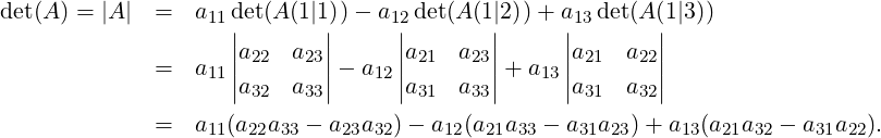
 ,
, 
 + 3
+ 3  = 4
= 4 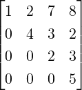


 ,
using Theorem
,
using Theorem  , det(
 ).
).
![[ ]
u v 2u + 3v](LA613x.png)


 = (
= ( + (
+ ( =
= 


 and det(
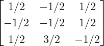 .
.


![( ( [ ] ) ) ( [ ]) ([ ])
- 1 C1 - 1 C1B -1 C1B
det(AB ) = det P B = det P = det(P ) ⋅det
0 0 0
= det(P) ⋅0 = 0 = 0 ⋅det(B) = det(A)det(B ).](LA664x.png)
![P Aj = P[A[:,1],...,A[:,j - 1],b, A[:,j + 1],...,A [:,n]]
= [P A[:,1],...,PA [:,j - 1],P b,P A[:,j + 1],...,P A[:,n ]]
= [e1,...,ej-1,d,ej+1,...,en].](LA684x.png)
 and
and  .
.