Definition 8.1.1. [Principal Minor] Let A ∈ Mn(ℂ).
- 1.
- Also, let S ⊆ [n]. Then, det
![(A [S, S])](LA2401x.png) is called the Principal minor of A corresponding
to S.
is called the Principal minor of A corresponding
to S.
- 2.
- By EMk(A), we denote the sum of all k × k principal minors of A.
We start this subsection with a few definitions and examples. So, it will be nice to recall the notations used in Section 1.3.1 and a few results from Appendix 9.2.
Definition 8.1.1. [Principal Minor] Let A ∈ Mn(ℂ).
is called the Principal minor of A corresponding
to S.
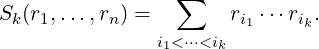
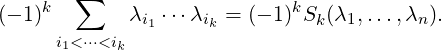
Definition 8.1.2. [Elementary Symmetric Functions] Let k be a positive integer. Then, the kth elementary symmetric function of the numbers r1,…,rn is Sk(r1,…,rn) and is defined as

 DRAFT
Example 8.1.3. Let A =
DRAFT
Example 8.1.3. Let A = 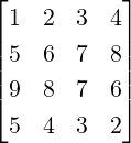 . Then, note that
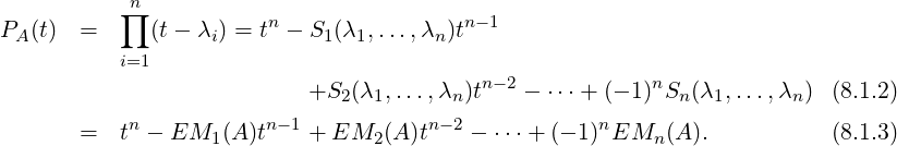
Proof. Note that by definition,
As the second part is just a re-writing of the first, we will just prove the first part. To do so, let B = tI - A =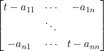 . Then, using Definition 9.2.2 in Appendix, note that
detB = ∑
σsgnσ ∏
i=1nbiσ(i) and hence each S ⊆ [n] with |S| = n - k has a contribution to the
coefficient of tn-k in the following way:
. Then, using Definition 9.2.2 in Appendix, note that
detB = ∑
σsgnσ ∏
i=1nbiσ(i) and hence each S ⊆ [n] with |S| = n - k has a contribution to the
coefficient of tn-k in the following way: For all i ∈ S, consider all permutations σ such that σ(i) = i. Our idea is to select a ‘t’ from these biσ(i). Since we do not want any more ‘t’, we set t = 0 for any other diagonal position. So the contribution from S to the coefficient of tn-k is det[-A(S|S)] = (-1)k detA(S|S). Hence the coefficient of tn-k in PA(t) is
![k ∑ k ∑ k
(- 1) detA(S |S ) = (- 1) detA [T,T] = (- 1) Ek (A ).
S⊆ [n],|S|=n-k T⊆[n],|T|=k](LA2411x.png)
As a direct application, we obtain Theorem 6.1.16 which we state again.

 DRAFT
DRAFT
Let A and B be similar matrices. Then, by Theorem 6.1.20, we know that σ(A) = σ(B). Thus, as a direct consequence of Part 2 of Theorem 8.1.4 gives the following result.
Corollary 8.1.6. Let A and B be two similar matrices of order n. Then, EMk(A) = EMk(B) for 1 ≤ k ≤ n.
So, the sum of principal minors of similar matrices are equal. Or in other words, the sum of principal minors are invariant under similarity.
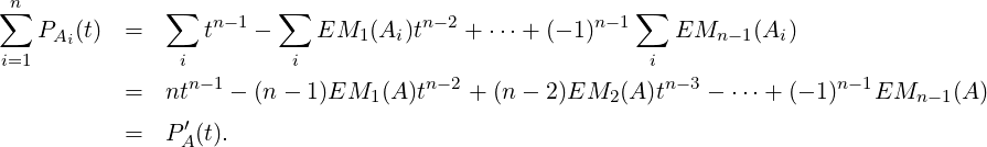
Proof. For 1 ≤ i ≤ n, let us denote A(i|i) by Ai. Then, using Equation (8.1.3), we have
Proof. As Alg.Mulα(A) = 1, PA(t) = (t - λ)q(t), where q(t) is a polynomial with q(λ)≠0. Thus P′A(t) = q(t) + (t - λ)q′(t). Hence, P′A(λ) = q(λ)≠0. Thus, by Corollary 8.1.7, ∑ iPA(i|i)(λ) = P′A(λ)≠0. Hence, there exists i,1 ≤ i ≤ n such that PA(i|i)(λ)≠0. That is, det[A(i|i) - λI]≠0 or Rank[A - λI] = n - 1. _
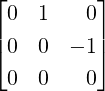
Remark 8.1.9. Converse of Corollary 8.1.8 is false. Note that for the matrix A = ![[ ]
0 1
0 0](LA2418x.png) ,
Rank[A - 0I] = 1 = 2 - 1 = n - 1, but 0 has multiplicity 2 as a root of PA(t) = 0.
,
Rank[A - 0I] = 1 = 2 - 1 = n - 1, but 0 has multiplicity 2 as a root of PA(t) = 0.
As an application of Corollary 8.1.7, we have the following result.
We now relate the multiplicity of an eigenvalue with the spectrum of a principal sub-matrix.
Theorem 8.1.10. [Multiplicity and Spectrum of a Principal Sub-Matrix] Let A ∈ Mn(ℂ) and k be a positive integer. Then 1 ⇒2 ⇒3, where

 DRAFT
DRAFT
Proof. Part 1⇒ Part 2. Let {x1,…,xk} be linearly independent eigenvectors for λ and let B be a
principal sub-matrix of A of size m > n-k. Without loss, we may write A = ![[ ]
B *
* *](LA2419x.png) . Let us partition
the xi’s , say xi =
. Let us partition
the xi’s , say xi = ![[ ]
x
i1
xi2](LA2420x.png) , such that
, such that
![[ | ][ ] [ ]
B |* xi1 = λ xi1 , for 1 ≤ i ≤ k.
* |* xi2 xi2](LA2423x.png)
![[ ]
y1
y2](LA2424x.png) of x1,…,xk such that y2 = 0.
Notice that y1≠0 and By1 = λy1.
of x1,…,xk such that y2 = 0.
Notice that y1≠0 and By1 = λy1.
Part 2⇒ Part 3. By Corollary 8.1.7, we know that P′A(t) = ∑
i=1nPA(i|i)(t). As A(i|i)
is of size n - 1, we get PA(i|i)(λ) = 0, for all i = 1,2,…,n. Thus, P′A(λ) = 0. A similar
argument now applied to each of the A(i|i)’s, gives PA(2)(λ) = 0, where PA(2)(t) =  P′A(t).
Proceeding on above lines, we finally get PA(i)(λ) = 0, for i = 0,1,…,k - 1. This implies that
Alg.Mulλ(A) ≥ k. _
P′A(t).
Proceeding on above lines, we finally get PA(i)(λ) = 0, for i = 0,1,…,k - 1. This implies that
Alg.Mulλ(A) ≥ k. _
Definition 8.1.11. [Moments] Fix a positive integer n and let α1,…,αn be n complex numbers. Then, for a positive integer k, the sum ∑ i=1nαik is called the k-th moment of the numbers α1,…,αn.
Theorem 8.1.12. [Newton’s identities] Let P(t) = tn + an-1tn-1 +  + a0 have zeros λ1,…,λn,
counted with multiplicities. Put μk = ∑
i=1nλik. Then, for 1 ≤ k ≤ n,
+ a0 have zeros λ1,…,λn,
counted with multiplicities. Put μk = ∑
i=1nλik. Then, for 1 ≤ k ≤ n,

 DRAFT
DRAFT
 | (8.1.4) |
That is, the first n moments of the zeros determine the coefficients of P(t).
Proof. For simplicity of expression, let an = 1. Then, using Equation (8.1.4), we see that k = 1 gives
us an-1 = -μ1. To compute an-2, put k = 2 in Equation (8.1.4) to verify that an-2 =  . This
process can be continued to get all the coefficients of P(t). Now, let us prove the n given
equations.
. This
process can be continued to get all the coefficients of P(t). Now, let us prove the n given
equations.
Define f(t) = ∑
i =
=  and take |t| > maxi|λi|. Then, the left hand side can be re-written
as
and take |t| > maxi|λi|. Then, the left hand side can be re-written
as
![n n n
∑ --1--- ∑ -(--1---)-- ∑ 1- λi n- μ1-
f(t) = t- λi = λi = [t + t2 + ⋅⋅⋅] = t + t2 + ⋅⋅⋅.
i=1 i=1 t 1 - t i=1](LA2433x.png) | (8.1.5) |
Thus, using P′(t) = f(t)P(t), we get
![n μ1
nantn-1 + (n - 1)an-1tn-2 + ⋅⋅⋅ + a1 = P ′(t) = [-+-2-+ ⋅⋅⋅][antn + ⋅⋅⋅+ a0].
t t](LA2434x.png)

 DRAFT
DRAFT

Remark 8.1.13. Let P(t) = antn +  + a1t + a0 with an = 1. Thus, we see that we need not
find the zeros of P(t) to find the k-th moments of the zeros of P(t). It can directly be computed
recursively using the Newton’s identities.
+ a1t + a0 with an = 1. Thus, we see that we need not
find the zeros of P(t) to find the k-th moments of the zeros of P(t). It can directly be computed
recursively using the Newton’s identities.
Exercise 8.1.14. Let A,B ∈ Mn(ℂ). Then, prove that A and B have the same eigenvalues if and only if tr(Ak) = tr(Bk), for k = 1,…,n. (Use Exercise 6.1.8 1a).
Let  = {A ∈ Mn(ℂ) : A*A = I}. Then, using Exercise 5.4.8, we see that
, AB ∈ (see Exercise 5.4.8.10).
, (AB)C = A(BC).
. That is, for any A ∈,AIn = A = InA.
,A-1 ∈.Thus, the set forma a group with respect to multiplication. We now define this group.

 DRAFT
Definition 8.2.1. [Unitary Group] Let = {A ∈ Mn(ℂ) : A*A = I}. Then, forms a
multiplicative group. This group is called the unitary group.
DRAFT
Definition 8.2.1. [Unitary Group] Let = {A ∈ Mn(ℂ) : A*A = I}. Then, forms a
multiplicative group. This group is called the unitary group.
Proposition 8.2.2. [Selection Principle of Unitary Matrices] Let {Uk : k ≥ 1} be a sequence of unitary matrices. Viewing them as elements of ℂn2 , let us assume that “for any ϵ > 0, there exists a positive integer N such that ∥Uk - U∥ < ϵ, for all k ≥ N”. That is, the matrices Uk’s converge to U as elements in ℂn2 . Then, U is also a unitary matrix.
Proof. Let A = [aij] ∈ Mn(ℂ) be an unitary matrix. Then ∑ i,j=1n|aij|2 = tr(A*A) = n. Thus, the set of unitary matrices is a compact subset of ℂn2 . Hence, any sequence of unitary matrices has a convergent subsequence (Bolzano-Weierstrass Theorem), whose limit is again unitary. Thus, the required result follows. _
For a unitary matrix U, we know that U-1 = U*. Our next result gives a necessary and sufficient condition on an invertible matrix A so that the matrix A-1 is similar to A*.
Theorem 8.2.3. [Generalizing a Unitary Matrix] Let A be an invertible matrix. Then A-1 is similar to A* if and only if there exists an invertible matrix B such that A = B-1B*.
Proof. Suppose A = B-1B*, for some invertible matrix B. Then

We first show that there exists a nonsingular Hermitian Hθ such that A-1 = Hθ-1A*Hθ, for some
θ ∈ ℝ.

 DRAFT
DRAFT
Note that for any θ ∈ ℝ, if we put Sθ = eiθS then


To get our result, we finally choose B = β(αI - A*)H(θ0) such that β≠0 and α = eiγ σ(A*).
Note that with α and β chosen as above, B is invertible. Furthermore,

Exercise 8.2.4. Suppose that A is similar to a unitary matrix. Then, prove that A-1 is similar
to A*.

 DRAFT
DRAFT
Definition 8.2.5. [Plane Rotations] For a fixed positive integer n, consider the vector space ℝn with standard basis {e1,…,en}. Also, for 1 ≤ i,j ≤ n, let Ei,j = eiejT . Then, for θ ∈ ℝ and 1 ≤ i,j ≤ n, a plane rotation, denoted U(θ;i,j), is defined as
![U (θ;i,j) = I - Ei,i - Ej,j + [Ei,i + Ej,j]cosθ - Ei,j sinθ + Ej,isinθ.](LA2450x.png)
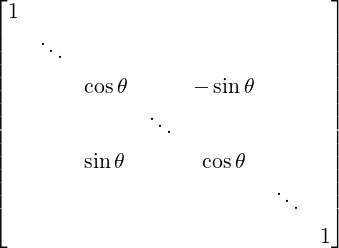 i j , where the unmentioned diagonal
entries are 1 and the unmentioned off-diagonal entries are 0.
i j , where the unmentioned diagonal
entries are 1 and the unmentioned off-diagonal entries are 0.
Remark 8.2.6. Note the following about the matrix U(θ;i,j), where θ ∈ ℝ and 1 ≤ i,j ≤ n.

 DRAFT
DRAFT
 T x rotates x by the angle -θ in the ij-plane.
 , whenever xj≠0.
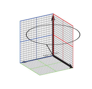
Then, we can either apply a plane rotation along the xy-plane or the yz-plane. For the xy-plane,
we need the plane z = 1 (xy plane lifted by 1). This plane contains the vector 1. Imagine moving
the tip of  on this plane. Then this locus corresponds to a circle that lies on the plane z = 1, has
radius
on this plane. Then this locus corresponds to a circle that lies on the plane z = 1, has
radius  and is centred at (0,0,1). That is, we draw the circle x2 + y2 = 1 on the
xy-plane and then lifted it up by so that it lies on the plane z = 1. Thus, note that the
xz-plane cuts this circle at two points. These two points of intersections give us the two
choices for the vector v (see Figure 8.1). A similar calculation can be done for the
yz-plane.
and is centred at (0,0,1). That is, we draw the circle x2 + y2 = 1 on the
xy-plane and then lifted it up by so that it lies on the plane z = 1. Thus, note that the
xz-plane cuts this circle at two points. These two points of intersections give us the two
choices for the vector v (see Figure 8.1). A similar calculation can be done for the
yz-plane.
 and it gets translated by
 ![[ ]
0, 0, a3, ⋅⋅⋅ an](LA2462x.png) T . So, there are two points x
on this circle with x2 = 0 and they are
T . So, there are two points x
on this circle with x2 = 0 and they are ![[ ]
±r, 0, a3, ⋅⋅⋅ an](LA2463x.png) T .
T .


 (1) =
(1) =  (1) = 0. Now, we can apply
an appropriate plane rotation U(θ3;2,3) so that U(θ3;2,3)
(1) = 0. Now, we can apply
an appropriate plane rotation U(θ3;2,3) so that U(θ3;2,3) = e2. Since e3 is the
only unit vector in ℝ3 orthogonal to both e1 and e2, it follows that U(θ3;2,3)
= e2. Since e3 is the
only unit vector in ℝ3 orthogonal to both e1 and e2, it follows that U(θ3;2,3) = e3.
Thus,
= e3.
Thus,
![[ ] [ ]
I = e1 e2 e3 = U(θ3;2,3)U (θ2;1,2)U (θ1;1,3) x y z .](LA2472x.png)
We are now ready to give another method to get the QR-decomposition of a square matrix (see Theorem 5.2.1 that uses the Gram-Schmidt Orthonormalization Process).
Proposition 8.2.7. [QR Factorization Revisited: Square Matrix] Let A ∈ Mn(ℝ). Then there exists a real orthogonal matrix Q and an upper triangular matrix R such that A = QR.
Proof. We start by applying the plane rotations to A so that the positions (2,1),(3,1),…,(n,1) of A become zero. This means, if a21 = 0, we multiply by I. Otherwise, we use the plane rotation U(θ;1,2), where θ = cot-1(-a11∕a21). Then, we apply a similar technique to A so that the (3,1) entry of A becomes 0. Note that this plane rotation doesn’t change the (2,1) entry of A. We continue this process till all the entry in the first column of A, except possibly the (1,1) entry, is zero.
We then apply the plane rotations to make positions (3,2),(4,2),…,(n,2) zero. Observe that this does not disturb the zeros in the first column. Thus, continuing the above process a finite number of times give us the required result. _

 DRAFT
Lemma 8.2.8. [QR Factorization Revisited: Rectangular Matrix] Let A ∈ Mm,n(ℝ). Then
there exists a real orthogonal matrix Q and a matrix R ∈ Mm,n(ℝ) in upper triangular form
such that A = QR.
DRAFT
Lemma 8.2.8. [QR Factorization Revisited: Rectangular Matrix] Let A ∈ Mm,n(ℝ). Then
there exists a real orthogonal matrix Q and a matrix R ∈ Mm,n(ℝ) in upper triangular form
such that A = QR.
Proof. If RankA < m, add some columns to A to get a matrix, say à such that Rankà = m. Now
suppose that à has k columns. For 1 ≤ i ≤ k, let vi = Ã[:,i]. Now, apply the Gram-Schmidt
Orthonormalization Process to {v1,…,vk}. For example, suppose the result is a sequence of k vectors
w1,0,w2,0,0,…,0,wm,0,…,0, where Q = ![[ ]
w1 ⋅⋅⋅ wm](LA2475x.png) is real orthogonal. Then Ã[:,1] is a linear
combination of w1, Ã[:,2] is also a linear combination of w1, Ã[:,3] is a linear combination of w1,w2
and so on. In general, for 1 ≤ s ≤ k, the column Ã[:,s] is a linear combination of wi-s in the list that
appear up to the s-th position. Thus, Ã[:,s] = ∑
i=1mwiris, where ris = 0 for all i > s. That is,
à = QR, where R = [rij]. Now, remove the extra columns of à and the corresponding columns in R to
get the required result. _
is real orthogonal. Then Ã[:,1] is a linear
combination of w1, Ã[:,2] is also a linear combination of w1, Ã[:,3] is a linear combination of w1,w2
and so on. In general, for 1 ≤ s ≤ k, the column Ã[:,s] is a linear combination of wi-s in the list that
appear up to the s-th position. Thus, Ã[:,s] = ∑
i=1mwiris, where ris = 0 for all i > s. That is,
à = QR, where R = [rij]. Now, remove the extra columns of à and the corresponding columns in R to
get the required result. _
Note that Proposition 8.2.7 is also valid for any complex matrix. In this case the matrix Q will be unitary. This can also be seen from Theorem 5.2.1 as we need to apply the Gram-Schmidt Orthonormalization Process to vectors in ℂn.
To proceed further recall that a matrix A = [aij] ∈ Mn(ℂ) is called a tri-diagonal matrix if aij = 0, whenever |i - j| > 1,1 ≤ i,j ≤ n.
Proposition 8.2.9. [Tridiagonalization of a Real Symmetric Matrix: Given’s Method] Let A be a real symmetric. Then, there exists a real orthogonal matrix Q such that QAQT is a tri-diagonal matrix.
Proof. If a31≠0, then put U1 = U(θ1;2,3), where θ1 = cot-1(-a21∕a31). Notice that U1T [:,1] = e1 and so
![(U1AU T1 )[:,1] = (U1A )[:,1].](LA2476x.png)

 DRAFT
DRAFT
![(U2 (U1AU T1 )U2T)[:,1) = (U2U1AU T1 )[:,1].](LA2479x.png)
![T T T
(U2U1AU 1 )[3,1] = U2[3,:](U1AU 1 )[:,1] = (U1AU 1 )[3,1] = 0.](LA2480x.png)
Continuing this way, we can find a real orthogonal matrix Q such that QAQT is tri-diagonal. _
Proposition 8.2.10. [Almost Diagonalization of a Real Symmetric Matrix: Jacobi method] Let A ∈ Mn(ℝ) be real symmetric. Then there exists a real orthogonal matrix S, a product of plane rotations, such that SAST is almost a diagonal matrix.
Proof. The idea is to reduce the off-diagonal entries of A to 0 as much as possible. So, we start with choosing i≠j) such that i < j and |aij| is maximum. Now, put


 DRAFT
DRAFT
![T T
blk = U [l,:]AU [:,k] = el Aek = alk
bik = UT [i,:]AU [:,k ] = (cosθeT + sin θeT)Aek = aikcosθ + ajksinθ
i j
blj = UT [l,:]AU [:,j] = eTl A (- sinθei + cosθej) = - alisinθ + alj cosθ
T T T
bij = U [i,:]AaUjj[-:,ajii] = (cos θei + sin θej )A(- sin θei + cosθej)
= sin(2θ)---2--+ aij cos(2θ) = 0](LA2484x.png)

We will now look at another class of unitary matrices, commonly called the Householder matrices (see Exercise 1.3.7.11).

 DRAFT
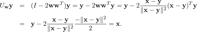
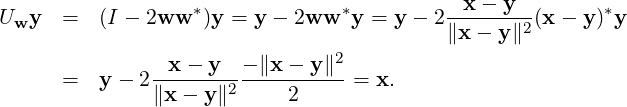
Definition 8.2.11. [Householder Matrix] Let w ∈ ℂn be a unit vector. Then, the matrix
Uw = I - 2ww* is called a Householder matrix.
DRAFT
Definition 8.2.11. [Householder Matrix] Let w ∈ ℂn be a unit vector. Then, the matrix
Uw = I - 2ww* is called a Householder matrix.
Remark 8.2.12. We observe the following about the Householder matrix Uw.
Example 8.2.13. In ℝ2, let w = e2. Then w⊥ is the x-axis. The vector v = ![[ ]
1
2](LA2489x.png) = e1 + 2e2,
where e1 ∈ w⊥ and 2e2 ∈ LS(w). So
= e1 + 2e2,
where e1 ∈ w⊥ and 2e2 ∈ LS(w). So

 DRAFT
DRAFT

Recall that if x,y ∈ ℝn with x≠y and ∥x∥ = ∥y∥ then, (x + y) ⊥ (x - y). This is not true
in ℂn as can be seen from the following example. Take x = ![[ ]
1
1](LA2493x.png) and y =
and y = ![[ ]
i
- 1](LA2494x.png) . Then
⟨
. Then
⟨![[ ]
1+ i
0](LA2495x.png) ,
,![[ ]
1- i
2](LA2496x.png) ⟩ = (1 + i)2≠0. Thus, to pick the right choice for the matrix Uw, we need to be
observant of the choice of the inner product space.
⟩ = (1 + i)2≠0. Thus, to pick the right choice for the matrix Uw, we need to be
observant of the choice of the inner product space.
Example 8.2.14. Let x,y ∈ ℂn with x≠y and ∥x∥ = ∥y∥. Then, which U
 ∈ ℝn. Then,

 DRAFT
DRAFT
 | (8.2.1) |
Furthermore, again using w*(y + x) = 0, we get y - x = 2ww*y = -2ww*x. So,

 = (y + x) [ww (y - x)] = (y + x) (y- x ).](LA2503x.png)
But, in that case, w =  will work as using above ∥x - y∥2 = 2(y - x)*y and
Thus, in this case, if ⟨x + y,x - y⟩≠0 then we will not find a w such that Uwy = x.
For example, taking x = ![[ ]
1
1](LA2508x.png) and y =
and y = ![[ ]
i
- 1](LA2509x.png) , we have ⟨x + y,x - y⟩≠0.
, we have ⟨x + y,x - y⟩≠0.
Proposition 8.2.15. [Householder’s Tri-Diagonalization] Let v ∈ ℝn-1 and A =
![[ ]
a vT
v B](LA2510x.png) ∈ Mn(ℝ) be a real symmetric matrix. Then, there exists a real orthogonal matrix Q,
a product of Householder matrices, such that QT AQ is tri-diagonal.
∈ Mn(ℝ) be a real symmetric matrix. Then, there exists a real orthogonal matrix Q,
a product of Householder matrices, such that QT AQ is tri-diagonal.
Proof. If v = e1 then we proceed to apply our technique to the matrix B, a matrix of lower order. So, without loss of generality, we assume that v≠e1.
As we want QT AQ to be tri-diagonal, we need to find a vector w ∈ ℝn-1 such that Uwv = re1 ∈ ℝn-1, where r = ∥v∥ = ∥Uwv∥. Thus, using Example 8.2.14, choose the required vector w ∈ ℝn-1. Then,
![⌊ ⌋
[ ][ ][ ] [ ] a r 0 [ ]
1 0 a vT 1 0 = a vTU Tw = | | = a reT1 ,
0 Uw v B 0 UTw Uwv UwBU Tw ⌈ r * *⌉ re1 S
0 * *](LA2511x.png)

 DRAFT
DRAFT
Definition 8.2.16. Let s and t be two symbols. Then, an expression of the form

Remark 8.2.17. [More on Unitary Equivalence] Let s and t be two symbols and W(s,t) be a word in symbols s and t.
Exercise 8.2.19. [Triangularization via Complex Orthogonal Matrix need not be Possible] Let A ∈ Mn(ℂ) and A = QTQT , where Q is complex orthogonal matrix and T is upper triangular. Then, prove that
![[ ]
1 i
i - 1](LA2517x.png) Q is upper triangular.
Q is upper triangular.Proposition 8.2.20. [Matrices with Distinct Eigenvalues are Dense in Mn(ℂ)] Let A ∈ Mn(ℂ). Then, for each ϵ > 0, there exists a matrix A(ϵ) ∈ Mn(ℂ) such that A(ϵ) = [a(ϵ)ij] has distinct eigenvalues and ∑ |aij - a(ϵ)ij|2 < ϵ.
Proof. By Schur Upper Triangularization (see Lemma 6.2.12), there exists a unitary matrix U such
that U*AU = T, an upper triangular matrix. Now, choose αi’s such that tii + αi are distinct
and ∑
|αi|2 < ϵ. Now, consider the matrix A(ϵ) = U U*. Then,
B = A(ϵ) - A = U diag(α1,…,αn)]U* with
U*. Then,
B = A(ϵ) - A = U diag(α1,…,αn)]U* with


 DRAFT
DRAFT
Before proceeding with our next result on almost diagonalizability, we look at the following example.
Example 8.2.21. Let A = ![[ ]
1 2
0 3](LA2522x.png) and ϵ > 0 be given. Then, determine a diagonal matrix D
such that the non-diagonal entry of D-1AD is less than ϵ.
and ϵ > 0 be given. Then, determine a diagonal matrix D
such that the non-diagonal entry of D-1AD is less than ϵ.
Solution: Choose α <  and define D = diag(1,α). Then,
![[ ][ ][ ] [ ]
D -1AD = 1 0 1 2 1 0 = 1 2α .
0 1α- 0 3 0 α 0 3](LA2524x.png)
 , the required result follows.
Proposition 8.2.22. [A matrix is Almost Diagonalizable] Let A ∈ Mn(ℂ) and ϵ > 0 be given. Then, there exists an invertible matrix Sϵ such that Sϵ-1ASϵ = T, an upper triangular matrix with |tij| < ϵ, for all i≠j.
Proof. By Schur Upper Triangularization (see Lemma 6.2.12), there exists a unitary matrix U such
that U*AU = T, an upper triangular matrix. Now, take t = 2 + maxi<j|tij| and choose α such
that 0 < α < ϵ∕t. Then, if we take Dα = diag(1,α,α2,…,αn-1) and S = UDα, we have
S-1AS = D TDα = F (say), an upper triangular. Furthermore, note that for i < j, we have
|fij| = |tij|αj-i ≤ ϵ. Thus, the required result follows. _
TDα = F (say), an upper triangular. Furthermore, note that for i < j, we have
|fij| = |tij|αj-i ≤ ϵ. Thus, the required result follows. _

 DRAFT
DRAFT
Definition 8.3.1. [Simultaneously Diagonalizable] Let A,B ∈ Mn(ℂ). Then, they are said to be simultaneously diagonalizable if there exists an invertible matrix S such that S-1AS and S-1BS are both diagonal matrices.
Since diagonal matrices commute, we have our next result.
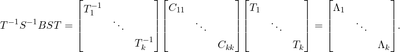
Proof. By definition, there exists an invertible matrix S such that S-1AS = Λ1 and S-1BS = Λ2. Hence,

Theorem 8.3.3. Let A,B ∈ Mn(ℂ) be diagonalizable matrices. Then they are simultaneously diagonalizable if and only if they commute.
Proof. One part of this theorem has already been proved in Proposition 8.3.2. For the other part, let us assume that AB = BA. Since A is diagonalizable, there exists an invertible matrix S such that

 DRAFT
DRAFT
 | (8.3.1) |
where λ1,…,λk are the distinct eigenvalues of A. We now use the sub-matrix structure of S-1AS to
decompose C = S-1BS as C = 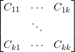 . Since AB = BA and S is invertible, we have
ΛC = CΛ. Thus,
. Since AB = BA and S is invertible, we have
ΛC = CΛ. Thus,
 ⊕ Ckk.
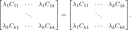
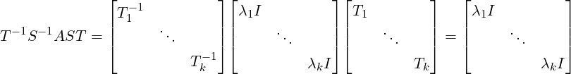
Since B is diagonalizable, the matrix C is also diagonalizable and hence the matrices Cii, for
1 ≤ i]lek, are diagonalizable. So, for 1 ≤ i ≤ k, there exists invertible matrices Ti’s such that
Ti-1CiiTi = Λi. Put T = T1 ⊕ ⊕ Tk. Then,

 DRAFT
DRAFT
Definition 8.3.4. [Commuting Family of Matrices]
 ⊆ Mn(ℂ). Then is said to be a commuting family if each pair of matrices in
commutes.
-invariant if W is B-invariant for each B ∈.
⊆ Mn(ℂ). Then is said to be a commuting family if each pair of matrices in
commutes.
-invariant if W is B-invariant for each B ∈.Example 8.3.5. Let A ∈ Mn(ℂ) with (λ,x) as an eigenpair. Then, W = {cx : c ∈ ℂ} is an A-invariant subspace. Furthermore, if W is an A-invariant subspace with dim(W) = 1 then verify that any non-zero vector in W is an eigenvector of A.
Theorem 8.3.6. [An A-invariant Subspace Contains an Eigenvector of A] Let A ∈ Mn(ℂ)
and W ⊆ ℂn be an A-invariant subspace of dimension at least 1. Then W contains an
eigenvector of A.

 DRAFT
DRAFT
Proof. Let  = {f1,…,fk}⊆ ℂn be an ordered basis for W. Define T : W → W as Tv = Av. Then
T[,] =
= {f1,…,fk}⊆ ℂn be an ordered basis for W. Define T : W → W as Tv = Av. Then
T[,] = ![[ ]
[Tf1]B ⋅⋅⋅ [T fk]B](LA2543x.png) is a k × k matrix which satisfies [Tw]
is a k × k matrix which satisfies [Tw] = T[,][w],
for all w ∈ W. As T[,] ∈ Mk(ℂ), it has an eigenpair, say (λ,
= T[,][w],
for all w ∈ W. As T[,] ∈ Mk(ℂ), it has an eigenpair, say (λ, ) with
  ∈ ℂk. That
is,
∈ ℂk. That
is,
![T [B, B]ˆx = λˆx.](LA2546x.png) | (8.3.2) |
Now, put x = ∑
i=1k( )ifi ∈ ℂn. Then, verify that x ∈ W and [x] =
  . Thus, Tx ∈ W and now
using Equation (8.3.2), we get
. Thus, Tx ∈ W and now
using Equation (8.3.2), we get
![∑ k ∑k ∑k ∑k ∑k
Tx = ([T x]B)ifi = (T[B,B ][x]B)ifi = (T [B, B]ˆx)ifi = (λˆx)ifi = λ (ˆx)ifi = λx.
i=1 i=1 i=1 i=1 i=1](LA2549x.png)
Theorem 8.3.7. Let ⊆ Mn(ℂ) be a commuting family of matrices. Then, all the matrices
in have a common eigenvector.
Proof. Note that ℂn is -invariant. Let W ⊆ ℂn be -invariant with minimum positive dimension. Let
y ∈ W such that y≠0. We claim that y is an eigenvector, for each A ∈.

 DRAFT
DRAFT
So, on the contrary assume y is not an eigenvector for some A ∈. Then, by Theorem 8.3.6, W
contains an eigenvector x of A for some eigenvalue, say λ. Define W0 = {z ∈ W : Az = λz}. So W0
is a proper subspace of W as y ∈ W \ W0. Also, for z ∈ W0 and C ∈, we note that
A(Cz) = CAz = λ(Cz), so that Cz ∈ W0. So W0 is -invariant and 1 ≤ dimW0 < dimW, a
contradiction. _
Theorem 8.3.8. Let ⊆ Mn(ℂ) be a family of diagonalizable matrices. Then is commuting
if and only if is simultaneously diagonalizable.
Proof. We prove the result by induction on n. The result is clearly true for n = 1. So, let us assume
the result to be valid for all n < m. Now, let us assume that ⊆ Mm(ℂ) is a family of diagonalizable
matrices.
If is simultaneously diagonalizable, then by Proposition 8.3.2, the family is commuting.
Conversely, let be a commuting family. If each A ∈ is a scalar matrix then they are
simultaneously diagonalizable via I. So, let A ∈ be a non-scalar matrix. As A is diagonalizable,
there exists an invertible matrix S such that
 = {
= { = S-1XS∣X ∈}. As is a commuting
family, the set is also a commuting family. So, each
= S-1XS∣X ∈}. As is a commuting
family, the set is also a commuting family. So, each  ∈ has the form
  = X1 ⊕
 ⊕Xk. Note
that
⊕Xk. Note
that  i = {Xi∣
 ∈} is a commuting family of diagonalizable matrices of size < m. Thus, by
induction hypothesis, i’s are simultaneously diagonalizable, say by the invertible matrices Ti’s.
That is, Ti-1XiTi = Λi, a diagonal matrix, for 1 ≤ i ≤ k. Thus, if T = T1 ⊕
∈} is a commuting family of diagonalizable matrices of size < m. Thus, by
induction hypothesis, i’s are simultaneously diagonalizable, say by the invertible matrices Ti’s.
That is, Ti-1XiTi = Λi, a diagonal matrix, for 1 ≤ i ≤ k. Thus, if T = T1 ⊕ ⊕ Tk
then
⊕ Tk
then
 . Thus the result holds by induction. _
We now give prove of some parts of Exercise 6.1.24.exe:eigen:1.
Remark 8.3.9. [σ(AB) and σ(BA)] Let m ≤ n, A ∈ Mm×n(ℂ), and B ∈ Mn×m(ℂ). Then σ(BA) = σ(AB) with n - m extra 0’s. In particular, if A,B ∈ Mn(ℂ) then, PAB(t) = PBA(t).
Proof. Note that
![[ ] [ ] [ ] [ ][ ]
AB 0 Im A AB ABA Im A 0 0
= = .
B 0 0 In B BA 0 In B BA](LA2562x.png)
![[ ]
AB 0
B 0](LA2563x.png) and
and ![[ ]
0 0
B BA](LA2564x.png) are similar. Hence, AB and BA have precisely the same
non-zero eigenvalues. Therefore, if they have the same size, they must have the same characteristic
polynomial. _
are similar. Hence, AB and BA have precisely the same
non-zero eigenvalues. Therefore, if they have the same size, they must have the same characteristic
polynomial. _
Exercise 8.3.10. [Miscellaneous Exercises]

 DRAFT
DRAFT
 and B =
  simultaneously triangularizable?
⊆ Mn(ℂ) be a family of commuting normal matrices. Then, prove that each element of
is simultaneously unitarily diagonalizable.
simultaneously triangularizable?
⊆ Mn(ℂ) be a family of commuting normal matrices. Then, prove that each element of
is simultaneously unitarily diagonalizable.
Proposition 8.3.11. [Triangularization: Real Matrix] Let A ∈ Mn(ℝ). Then, there exists a
real orthogonal matrix Q such that QT AQ is block upper triangular, where each diagonal block
is of size either 1 or 2.

 DRAFT
DRAFT
Proof. If all the eigenvalues of A are real then the corresponding eigenvectors have real entries and hence, one can use induction to get the result in this case (see Lemma 6.2.12).
So, now let us assume that A has a complex eigenvalue, say λ = α + iβ with β≠0 and x = u + iv as an eigenvector for λ. Thus, Ax = λx and hence Ax = λx. But, λ≠λ as β≠0. Thus, the eigenvectors x,x are linearly independent and therefore, {u,v} is a linearly independent set. By Gram-Schmidt Orthonormalization process, we get an ordered basis, say {w1,w2,…,wn} of ℝn, where LS(w1,w2) = LS(u,v). Also, using the eigen-condition Ax = λx gives

Now, form a matrix X = ![[w1, w2,...,wn ]](LA2572x.png) . Then, X is a real orthogonal matrix and
. Then, X is a real orthogonal matrix and
The next result is a direct application of Proposition 8.3.11 and hence the proof is omitted.

 DRAFT
Corollary 8.3.12. [Simultaneous Triangularization: Real Matrices] Let ⊆ Mn(ℝ) be a
commuting family. Then, there exists a real orthogonal matrix Q such that QT AQ is a block
upper triangular matrix, where each diagonal block is of size either 1 or 2, for all A ∈.
DRAFT
Corollary 8.3.12. [Simultaneous Triangularization: Real Matrices] Let ⊆ Mn(ℝ) be a
commuting family. Then, there exists a real orthogonal matrix Q such that QT AQ is a block
upper triangular matrix, where each diagonal block is of size either 1 or 2, for all A ∈.
Proposition 8.3.13. Let A ∈ Mn(ℝ). Then the following statements are equivalent.
Proof. 2 ⇒ 1 is trivial. To prove 1 ⇒ 2, recall that Proposition 8.3.11 gives the existence of a real orthogonal matrix Q such that QT AQ is upper triangular with diagonal blocks of size either 1 or 2. So, we can write
![⌊ | ⌋
|λ1 *. * |* * * |
||0 .. * |* * * || [ ]
||0 ⋅⋅⋅ λp |* * * || R C
QT AQ = ||-----------|-------------|| = (say).
|0 ⋅⋅⋅ 0 |A11 ⋅.⋅⋅ A1k| 0 B
|⌈0 ⋅⋅⋅ 0 |0 .. * |⌉
0 ⋅⋅⋅ 0 |0 ⋅⋅⋅ Akk](LA2576x.png)
![[ ]
R C
0 B](LA2577x.png)
![[ ]
RT 0
T T
C B](LA2578x.png) =
= ![[ ]
RT 0
T T
C B](LA2579x.png)
![[ ]
R C
0 B](LA2580x.png) . Thus, tr(CCT ) = tr(RRT -RT R) = 0. Now,
using Exercise 8.3.10.9, we get C = 0. Hence, RRT = RT R and therefore, R is a diagonal
matrix.
. Thus, tr(CCT ) = tr(RRT -RT R) = 0. Now,
using Exercise 8.3.10.9, we get C = 0. Hence, RRT = RT R and therefore, R is a diagonal
matrix.

 DRAFT
DRAFT
As BT B = BBT , we have ∑
A1iA1iT = A11A11T . So tr ∑
2kA1iA1iT
∑
2kA1iA1iT  = 0. Now, using
Exercise 8.3.10.9 again, we have ∑
2kA1iA1iT = 0 and so A1iA1iT = 0, for all i = 2,…,k. Thus,
A1i = 0, for all i = 2,…,k. Hence, the required result follows. _
= 0. Now, using
Exercise 8.3.10.9 again, we have ∑
2kA1iA1iT = 0 and so A1iA1iT = 0, for all i = 2,…,k. Thus,
A1i = 0, for all i = 2,…,k. Hence, the required result follows. _
Exercise 8.3.14. Let A ∈ Mn(ℝ). Then the following are true.
![[ ]
0 a
i
- ai 0](LA2585x.png) , for some real numbers ai’s.
, for some real numbers ai’s.
![[ cosθ sin θ ]
j j
- sinθj cosθj](LA2586x.png) , for some real numbers θi’s.
, for some real numbers θi’s.
Definition 8.3.15. [Convergent matrices] A matrix A is called a convergent matrix if Am → 0 as m →∞.
Proof. Let A = U* diag(λ1,…,λn)U. As ρ(A) < 1, for each i,1 ≤ i ≤ n, λim → 0 as
m →∞. Thus, Am = U* diag(λ1m,…,λnm)U → 0. _

 DRAFT
DRAFT
Proof. Let Jk(λ) = λIk + Nk be a Jordan block of J = Jordan CFA. Then as Nkk = 0, for each fixed k, we have

Conversely, if A is convergent, then J must be convergent. Thus each Jordan block Jk(λ) must be convergent. Hence |λ| < 1. _
Theorem 8.3.17. [Decomposition into Diagonalizable and Nilpotent Parts] Let A ∈ Mn(ℂ). Then A = B + C, where B is diagonalizable matrix and C is nilpotent such that BC = CB.
Proof. Let J = Jordan CFA. Then, J = D + N, where D = diag(J) and N is clearly a nilpotent matrix.
Now, note that DN = ND as for each Jordan block Jk(λ) = Dk + Nk, we have Dk = λI and
Nk = Jk(0) so that DkNk = NkDk. As J = Jordan CFA, there exists an invertible matrix S, such
that S-1AS = J. Hence, A = SJS-1 = SDS-1 + SNS-1 = B + C, which satisfy the required
conditions. _

 DRAFT
DRAFT

 DRAFT
DRAFT

 DRAFT
DRAFT


![⌊ ⌋
w *1
| *|
X *AX = X *[Aw ,Aw ,...,Aw ] = ||w 2|| [aw + bw ,cw + dw ,...,Aw ]
1 2 n |⌈ ... |⌉ 1 2 1 2 n
*
w n
⌊ a b ⌋
| * |
= ⌈ c d ⌉ (8.3.3)
0 B](LA2573x.png)