Definition 9.1.1. Fix n ∈ ℕ. Then, for each f ∈ n, we associate an n × n matrix, denoted
Pf = [pij], such that pij = 1, whenver f(j) = i and 0, otherwise. The matrix Pf is called the
Permutation matrix corresponding to the permutation f. For example, I2, corresponding
to Id2, and
n, we associate an n × n matrix, denoted
Pf = [pij], such that pij = 1, whenver f(j) = i and 0, otherwise. The matrix Pf is called the
Permutation matrix corresponding to the permutation f. For example, I2, corresponding
to Id2, and ![[ ]
0 1
1 0](LA2598x.png) = E12, corresponding to the permutation (1,2), are the two permutation
matrices of order 2 × 2.
= E12, corresponding to the permutation (1,2), are the two permutation
matrices of order 2 × 2.
Remark 9.1.2. Recall that in Remark 9.2.16.1, it was observed that each permutation is a product of
n transpositions, (1,2),…,(1,n).
-
1.
- Verify that the elementary matrix Eij is the permutation matrix corresponding to the
transposition (i,j) .
-
2.
- Thus, every permutation matrix is a product of elementary matrices E1j, 1 ≤ j ≤ n.
-
3.
- For n = 3, the permutation matrices are I3,
 = E
23 = E12E13E12,
= E
23 = E12E13E12,
 = E
12,
= E
12,  = E
12E13,
= E
12E13,  = E
13E12 and
= E
13E12 and  = E
13.
= E
13.
-
4.
- Let f ∈ n and Pf = [pij] be the corresponding permutation matrix. Since pij = δi,j
and {f(1),…,f(n)} = [n], each entry of Pf is either 0 or 1. Furthermore, every row and
column of Pf has exactly one nonzero entry. This nonzero entry is a 1 and appears at the
position pi,f(i).
-
5.
- By the previous paragraph, we see that when a permutation matrix is multiplied to A

 DRAFT
DRAFT
-
(a)
- from left then it permutes the rows of A.
-
(b)
- from right then it permutes the columns of A.
-
6.
- P is a permutation matrix if and only if P has exactly one 1 in each row and column.
Solution: If P has exactly one 1 in each row and column, then P is a square matrix, say n×n.
Now, apply GJE to P. The occurrence of exactly one 1 in each row and column implies that
these 1’s are the pivots in each column. We just need to interchange rows to get it in RREF. So,
we need to multiply by Eij. Thus, GJE of P is In and P is indeed a product of Eij’s. The other
part has already been explained earlier.
We are now ready to prove Theorem 2.2.17.
Theorem 9.1.3. Let A and B be two matrices in RREF. If they are row equivalent then
A = B.
Proof. Note that the matrix A = 0 if and only if B = 0. So, let us assume that the matrices A,B≠0.
Also, the row-equivalence of A and B implies that there exists an invertible matrix C such that
A = CB, where C is product of elementary matrices.
Since B is in RREF, either B[:,1] = 0T or B[:,1] = (1,0,…,0)T . If B[:,1] = 0T then
A[:,1] = CB[:,1] = C0 = 0. If B[:,1] = (1,0,…,0)T then A[:,1] = CB[:,1] = C[:,1]. As C is invertible,
the first column of C cannot be the zero vector. So, A[:,1] cannot be the zero vector. Further, A is in
RREF implies that A[:,1] = (1,0,…,0)T . So, we have shown that if A and B are row-equivalent then
their first columns must be the same.
Now, let us assume that the first k - 1 columns of A and B are equal and it contains r pivotal
columns. We will now show that the k-th column is also the same.
Define Ak = [A[:,1],…,A[:,k]] and Bk = [B[:,1],…,B[:,k]]. Then, our assumption implies that
A[:,i] = B[:,i], for 1 ≤ i ≤ k - 1. Since, the first k - 1 columns contain r pivotal columns, there exists
a permutation matrix P such that

 DRAFT
DRAFT
![[ | ] [ | ]
Ir W |A[:,k] Ir W |B [:,k]
AkP = | and BkP = | .
0 0 | 0 0 |](LA2606x.png)
If the k-th columns of A and B are pivotal columns then by definition of RREF,
A[:,k] = ![[ ]
0
e1](LA2609x.png) = B[:,k], where 0 is a vector of size r and e1 = (1,0,…,0)T . So, we need to consider
two cases depending on whether both are non-pivotal or one is pivotal and the other is
not.
= B[:,k], where 0 is a vector of size r and e1 = (1,0,…,0)T . So, we need to consider
two cases depending on whether both are non-pivotal or one is pivotal and the other is
not.
As A = CB, we get Ak = CBk and
![[ | ] [ | ][ | ] [ | ]
Ir W |A[:,k] C1 |C2 Ir W |B [:,k] C1 C1W |CB [:,k]
| = AkP = CBkP = | | = | .
0 0 | C3 |C4 0 0 | C3 C3W |](LA2610x.png) So,
we see that C1 = Ir, C3 = 0 and A[:,k] =
So,
we see that C1 = Ir, C3 = 0 and A[:,k] = ![[ | ]
Ir |C2
0 |C
4](LA2611x.png) B[:,k].
B[:,k].
Case 1: Neither A[:,k] nor B[:,k] are pivotal. Then
![[ ] [ | ] [ | ] [ ] [ ]
X = A[:,k] = Ir |C2 B[:,k ] = Ir |C2 Y = Y .
0 0 |C4 0 |C4 0 0](LA2612x.png) Thus, X = Y and in this case the k-th columns are equal.
Thus, X = Y and in this case the k-th columns are equal.
Case 2: A[:,k] is pivotal but B[:,k] in non-pivotal. Then
![[ ] [ | ] [ | ] [ ] [ ]
0 Ir |C2 Ir |C2 Y Y
e1 = A [:,k] = 0 |C4 B[:,k] = 0 |C4 0 = 0 ,](LA2613x.png) a
contradiction as e1≠0. Thus, this case cannot arise.
a
contradiction as e1≠0. Thus, this case cannot arise.
Therefore, combining both the cases, we get the required result. _
Definition 9.2.1. For a positive integer n, denote [n] = {1,2,…,n}. A function f : A → B is called
-
1.
- one-one/injective if f(x) = f(y) for some x,y ∈ A necessarily implies that x = y.
-
2.
- onto/surjective if for each b ∈ B there exists a ∈ A such that f(a) = b.
-
3.
- a bijection if f is both one-one and onto.
Example 9.2.2. Let A = {1,2,3}, B = {a,b,c,d} and C = {α,β,γ}. Then, the function
-
1.
- j : A → B defined by j(1) = a,j(2) = c and j(3) = c is neither one-one nor onto.
-
2.
- f : A → B defined by f(1) = a,f(2) = c and f(3) = d is one-one but not onto.
-
3.
- g : B → C defined by g(a) = α,g(b) = β,g(c) = α and g(d) = γ is onto but not one-one.
-
4.
- h : B → A defined by h(a) = 2,h(b) = 2,h(c) = 3 and h(d) = 1 is onto.
-
5.
- h ∘ f : A → A is a bijection.

 DRAFT
DRAFT
-
6.
- g ∘ f : A → C is neither one-one not onto.
Remark 9.2.3. Let f : A → B and g : B → C be functions. Then, the composition of
functions, denoted g ∘ f, is a function from A to C defined by (g ∘ f)(a) = g(f(a)). Also, if
-
1.
- f and g are one-one then g ∘ f is one-one.
-
2.
- f and g are onto then g ∘ f is onto.
Thus, if f and g are bijections then so is g ∘ f.
Definition 9.2.4. A function f : [n] → [n] is called a permutation on n elements if f is a
bijection. For example, f,g : [2] → [2] defined by f(1) = 1,f(2) = 2 and g(1) = 2,g(2) = 1 are
permutations.
Remark 9.2.6. Let f : [n] → [n] be a bijection. Then, the inverse of f, denote f-1, is defined
by f-1(m) = ℓ whenever f(ℓ) = m for m ∈ [n] is well defined and f-1 is a bijection. For
example, in Exercise 9.2.5, note that fi-1 = fi, for i = 1,2,3,6 and f4-1 = f5.
Remark 9.2.7. Let n = {f : [n] → [n] : σ is a permutation}. Then, n has n! elements
and forms a group with respect to composition of functions, called product, due to the
following.
-
1.
- Let f ∈ Sn. Then,
-
(a)
- f can be written as f =
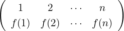 , called a two row notation.
-
(b)
- f is one-one. Hence, {f(1),f(2),…,f(n)} = [n] and thus, f(1) ∈ [n],f(2) ∈
[n] \{f(1)},… and finally f(n) = [n] \{f(1),…,f(n - 1)}. Therefore, there are n
choices for f(1), n- 1 choices for f(2) and so on. Hence, the number of elements in
n equals n(n - 1)
 2 ⋅ 1 = n!.
-
2.
- By Remark 9.2.3, f ∘ g ∈n, for any f,g ∈ Sn.
-
3.
- Also associativity holds as f ∘ (g ∘ h) = (f ∘ g) ∘ h for all functions f,g and h.
-
4.
- n has a special permutation called the identity permutation, denoted Idn, such that Idn(i) = i,
for 1 ≤ i ≤ n.

 DRAFT
DRAFT
-
5.
- For each f ∈n, f-1 ∈n and is called the inverse of f as f ∘ f-1 = f-1 ∘ f = Idn.
Proof. Part 1: Note that for each α ∈n the functions f-1∘α,α∘f-1 ∈n and α = f∘(f-1∘α)
as well as α = (α ∘ f-1) ∘ f.
Part 2: Note that for each f ∈n, by definition, (f-1)-1 = f. Hence the result holds. __
Definition 9.2.9. Let f ∈n. Then, the number of inversions of f, denoted n(f), equals
Example 9.2.10.
-
1.
- For f =
 , n(f) = |{(1,2),(1,3),(2,3)}| = 3.
-
2.
- In Exercise 9.2.5, n(f5) = 2 + 0 = 2.
-
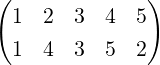
3.
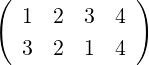
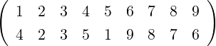
- Let f =
 . Then, n(f) = 3+1+1+1+0+3+2+1 = 12.
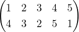
Definition 9.2.11. [Cycle Notation] Let f ∈ n. Suppose there exist r,2 ≤ r ≤ n and
i1,…,ir ∈ [n] such that f(i1) = i2,f(i2) = i3,…,f(ir) = i1 and f(j) = j for all j≠i1,…,ir.
Then, we represent such a permutation by f = (i1,i2,…,ir) and call it an r-cycle. For example,
f = 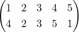 = (1,4,5) and
 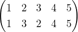 = (2,3).
Remark 9.2.12.
-
1.
- One also write the r-cycle (i1,i2,…,ir) as (i2,i3,…,ir,i1) and so on. For example, (1,4,5) =
(4,5,1) = (5,1,4).

 DRAFT
DRAFT
-
2.
- The permutation f =
 is not a cycle.
-
3.
- Let f = (1,3,5,4) and g = (2,4,1) be two cycles. Then, their product, denoted f ∘ g or
(1,3,5,4)(2,4,1) equals (1,2)(3,5,4). The calculation proceeds as (the arrows indicate the
images):
1 → 2. Note (f ∘ g)(1) = f(g(1)) = f(2) = 2.
2 → 4 → 1 as (f ∘ g)(2) = f(g(2)) = f(4) = 1. So, (1,2) forms a cycle.
3 → 5 as (f ∘ g)(3) = f(g(3)) = f(3) = 5.
5 → 4 as (f ∘ g)(5) = f(g(5)) = f(5) = 4.
4 → 1 → 3 as (f ∘ g)(4) = f(g(4)) = f(1) = 3. So, the other cycle is (3,5,4).
-
4.
- Let f = (1,4,5) and g = (2,4,1) be two permutations. Then, (1,4,5)(2,4,1) =
(1,2,5)(4) = (1,2,5) as 1 → 2,2 → 4 → 5,5 → 1,4 → 1 → 4 and
(2,4,1)(1,4,5) = (1)(2,4,5) = (2,4,5) as 1 → 4 → 1,2 → 4,4 → 5,5 → 1 → 2.
-
5.
- Even though
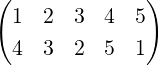 is not a cycle, verify that it is a product of the cycles
(1,4,5) and (2,3).
is not a cycle, verify that it is a product of the cycles
(1,4,5) and (2,3).
Definition 9.2.13. A permutation f ∈n is called a transposition if there exist m,r ∈ [n]
such that f = (m,r).
Remark 9.2.14. Verify that
-
1.
- (2,4,5) = (2,5)(2,4) = (4,2)(4,5) = (5,4)(5,2) = (1,2)(1,5)(1,4)(1,2).
-
2.
- in general, the r-cycle (i1,…,ir) = (1,i1)(1,ir)(1,ir-1)
 (1,i2)(1,i1).
-
3.
- So, every r-cycle can be written as product of transpositions. Furthermore, they can be
written using the n transpositions (1,2),(1,3),…,(1,n).

 DRAFT
DRAFT
With the above definitions, we state and prove two important results.
Theorem 9.2.15. Let f ∈n. Then, f can be written as product of transpositions.
Proof. Note that using use Remark 9.2.14, we just need to show that f can be written as
product of disjoint cycles.
Consider the set S = {1,f(1),f(2)(1) = (f ∘ f)(1),f(3)(1) = (f ∘ (f ∘ f))(1),…}. As S is an
infinite set and each f(i)(1) ∈ [n], there exist i,j with 0 ≤ i < j ≤ n such that f(i)(1) = f(j)(1).
Now, let j1 be the least positive integer such that f(i)(1) = f(j1)(1), for some i,0 ≤ i < j1.
Then, we claim that i = 0.
For if, i - 1 ≥ 0 then j1 - 1 ≥ 1 and the condition that f is one-one gives

Thus, we see that the repetition has occurred at the (
j1 - 1)-th instant, contradicting the
assumption that
j1 was the least such positive integer. Hence, we conclude that
i = 0. Thus,
(1
,f(1)
,f(2)(1)
,…,f(j1-1)(1)) is one of the cycles in
f.
Now, choose i1 ∈ [n] \{1,f(1),f(2)(1),…,f(j1-1)(1)} and proceed as above to get another
cycle. Let the new cycle by (i1,f(i1),…,f(j2-1)(i1)). Then, using f is one-one follows that

 DRAFT
DRAFT

So, the above process needs to be repeated at most
n times to get all the disjoint cycles. Thus,
the required result follows. __
Remark 9.2.16. Note that when one writes a permutation as product of disjoint cycles, cycles of
length 1 are suppressed so as to match Definition 9.2.11. For example, the algorithm in the proof of
Theorem 9.2.15 implies
-
1.
- Using Remark 9.2.14.3, we see that every permutation can be written as product of the
n transpositions (1,2),(1,3),…,(1,n).
-
2.
 = (1)(2,4,5)(3) = (2,4,5).
-
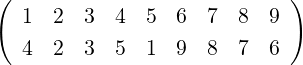
3.
 = (1,4,5)(2)(3)(6,9)(7,8) = (1,4,5)(6,9)(7,8).
Note that Id3 = (1,2)(1,2) = (1,2)(2,3)(1,2)(1,3), as well. The question arises, is it possible to
write Idn as a product of odd number of transpositions? The next lemma answers this question in
negative.
Proof. We will prove the result by mathematical induction. Observe that t≠1 as Idn is not a
transposition. Hence, t ≥ 2. If t = 2, we are done. So, let us assume that the result holds for all
expressions in which the number of transpositions t ≤ k. Now, let t = k + 1.
Suppose f1 = (m,r) and let ℓ,s ∈ [n] \ {m,r}. Then, the possible choices for the
composition f1 ∘ f2 are (m,r)(m,r) = Idn,(m,r)(m,ℓ) = (r,ℓ)(r,m),(m,r)(r,ℓ) = (ℓ,r)(ℓ,m)
and (m,r)(ℓ,s) = (ℓ,s)(m,r). In the first case, f1 and f2 can be removed to obtain Idn =
f3 ∘f4 ∘ ∘ft, where the number of transpositions is t- 2 = k - 1 < k. So, by mathematical
induction, t - 2 is even and hence t is also even.
∘ft, where the number of transpositions is t- 2 = k - 1 < k. So, by mathematical
induction, t - 2 is even and hence t is also even.
In the remaining cases, the expression for f1 ∘ f2 is replaced by their counterparts to
obtain another expression for Idn. But in the new expression for Idn, m doesn’t appear in
the first transposition, but appears in the second transposition. The shifting of m to the right
can continue till the number of transpositions reduces by 2 (which in turn gives the result
by mathematical induction). For if, the shifting of m to the right doesn’t reduce the number
of transpositions then m will get shifted to the right and will appear only in the right most
transposition. Then, this expression for Idn does not fix m whereas Idn(m) = m. So, the later
case leads us to a contradiction. Hence, the shifting of m to the right will surely lead to an
expression in which the number of transpositions at some stage is t - 2 = k - 1. At this stage,
one applies mathematical induction to get the required result. __
Proof. As g1 ∘ ∘ gk = h1 ∘
 ∘ hℓ and h-1 = h for any transposition h ∈n, we have

Hence by Lemma
9.2.17,
k +
ℓ is even. Thus, either
k and
ℓ are both even or both odd. __
Definition 9.2.19. [Even and Odd Permutation] A permutation f ∈n is called an
-
1.
- even permutation if f can be written as product of even number of transpositions.
-
2.
- odd permutation if f can be written as a product of odd number of transpositions.
Example 9.2.21. Consider the set n. Then,
-
1.
- by Lemma 9.2.17, Idn is an even permutation and sgn(Idn) = 1.
-
2.
- a transposition, say f, is an odd permutation and hence sgn(f) = -1
-
3.
- using Remark 9.2.20, sgn(f ∘ g) = sgn(f) ⋅ sgn(g) for any two permutations f,g ∈n.
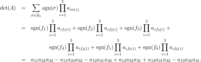
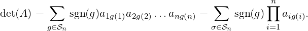
We are now ready to define determinant of a square matrix A.
Observe that det(A) is a scalar quantity. Even though the expression for det(A) seems complicated
at first glance, it is very helpful in proving the results related with “properties of determinant”. We
will do so in the next section. As another examples, we verify that this definition also
matches for 3 × 3 matrices. So, let A = [aij] be a 3 × 3 matrix. Then, using Equation (9.2.2),
Theorem 9.3.1 (Properties of Determinant). Let A = [aij] be an n × n matrix.
-
1.
- If A[i,:] = 0T for some i then det(A) = 0.
-
2.
- If B = Ei(c)A, for some c≠0 and i ∈ [n] then det(B) = cdet(A).

 DRAFT
DRAFT
-
3.
- If B = EijA, for some i≠j then det(B) = -det(A).
-
4.
- If A[i,:] = A[j,:] for some i≠j then det(A) = 0.
-
5.
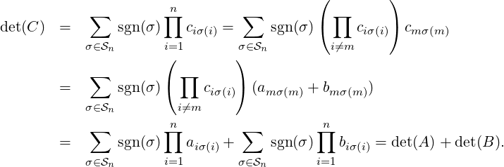
- Let B and C be two n×n matrices. If there exists m ∈ [n] such that B[i,:] = C[i,:] = A[i,:]
for all i≠m and C[m,:] = A[m,:] + B[m,:] then det(C) = det(A) + det(B).
-
6.
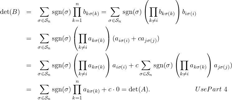
- If B = Eij(c), for c≠0 then det(B) = det(A).
-
7.
- If A is a triangular matrix then det(A) = a11
 ann, the product of the diagonal entries.
-
8.
- If E is an n × n elementary matrix then det(EA) = det(E)det(A).
-
9.
- A is invertible if and only if det(A)≠0.
-
10.
- If B is an n × n matrix then det(AB) = det(A)det(B).
-
11.
- If AT denotes the transpose of the matrix A then det(A) = det(AT ).
Proof. Part 1: Note that each sum in det(A) contains one entry from each row. So, each sum
has an entry from A[i,:] = 0T . Hence, each sum in itself is zero. Thus, det(A) = 0.
Part 2: By assumption, B[k,:] = A[k,:] for k≠i and B[i,:] = cA[i,:]. So,
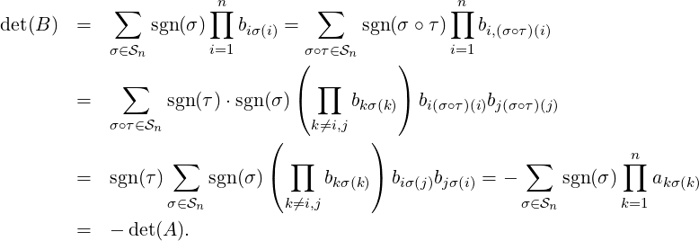
Part 3: Let τ = (i,j). Then, sgn(τ) = -1, by Lemma 9.2.8, n = {σ ∘ τ : σ ∈n} and
Part 4: As A[i,:] = A[j,:], A = EijA. Hence, by Part 3, det(A) = -det(A). Thus, det(A) = 0.
Part 5: By assumption, C[i,:] = B[i,:] = A[i,:] for i≠m and C[m,:] = B[m,:] + A[m,:]. So,
Part 6: By assumption, B[k,:] = A[k,:] for k≠i and B[i,:] = A[i,:] + cA[j,:]. So,
Part 7: Observe that if σ ∈n and σ≠Idn then n(σ) ≥ 1. Thus, for every σ≠Idn, there
exists m ∈ [n] (depending on σ) such that m > σ(m) or m < σ(m). So, if A is triangular,
amσ(m) = 0. So, for each σ≠Idn, ∏
i=1naiσ(i) = 0. Hence, det(A) = ∏
i=1naii. the result
follows.
Part 8: Using Part 7, det(In) = 1. By definition Eij = EijIn and Ei(c) = Ei(c)In and
Eij(c) = Eij(c)In, for c≠0. Thus, using Parts 2, 3 and 6, we get det(Ei(c)) = c,det(Eij) = -1 and
det(Eij(k)) = 1. Also, again using Parts 2, 3 and 6, we get det(EA) = det(E)det(A).
Part 9: Suppose A is invertible. Then, by Theorem 2.3.1, A = E1 Ek, for some elementary matrices
E1,…,Ek. So, a repeated application of Part 8 implies det(A) = det(E1)
Ek, for some elementary matrices
E1,…,Ek. So, a repeated application of Part 8 implies det(A) = det(E1) det(Ek)≠0 as det(Ei)≠0
for 1 ≤ i ≤ k.
det(Ek)≠0 as det(Ei)≠0
for 1 ≤ i ≤ k.

 DRAFT
DRAFT
Now, suppose that det(A)≠0. We need to show that A is invertible. On the contrary, assume that
A is not invertible. Then, by Theorem 2.3.1, Rank(A) < n. So, by Proposition 2.2.21, there exist
elementary matrices E1,…,Ek such that E1 EkA =
EkA = ![[ ]
B
0](LA2676x.png) . Therefore, by Part 1 and a repeated
application of Part 8 gives
. Therefore, by Part 1 and a repeated
application of Part 8 gives
![( [ ])
B
det(E1)⋅⋅⋅det(Ek)det(A ) = det(E1 ⋅⋅⋅EkA ) = det = 0.
0](LA2679x.png)
As
det(
Ei)
≠0, for 1
≤ i ≤ k, we have det(
A) = 0, a contradiction. Thus,
A is invertible.
Part 10: Let A be invertible. Then, by Theorem 2.3.1, A = E1 Ek, for some elementary
matrices E1,…,Ek. So, applying Part 8 repeatedly gives det(A) = det(E1)
Ek, for some elementary
matrices E1,…,Ek. So, applying Part 8 repeatedly gives det(A) = det(E1) det(Ek)
and
det(Ek)
and

In case A is not invertible, by Part 9, det(A) = 0. Also, AB is not invertible (AB is invertible will
imply A is invertible using the rank argument). So, again by Part 9, det(AB) = 0. Thus,
det(AB) = det(A)det(B).
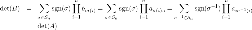
Part 11: Let B = [bij] = AT . Then, bij = aji, for 1 ≤ i,j ≤ n. By Lemma 9.2.8, we know that
n = {σ-1 : σ ∈n}. As σ ∘ σ-1 = Idn, sgn(σ) = sgn(σ-1). Hence,
__
Remark 9.3.2.
-
1.
- As det(A) = det(AT ), we observe that in Theorem 9.3.1, the condition on “row” can be
replaced by the condition on “column”.
-
2.
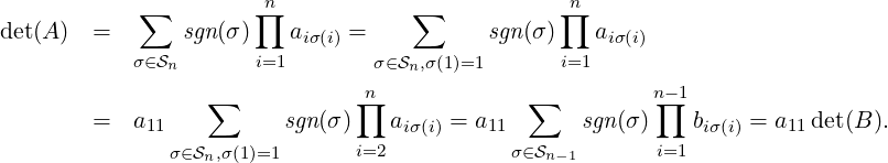
- Let A = [aij] be a matrix satisfying a1j = 0, for 2 ≤ j ≤ n. Let B = A(1|1), the submatrix of A
obtained by removing the first row and the first column. Then det(A) = a11 det(B).
Proof: Let σ ∈n with σ(1) = 1. Then, σ has a cycle (1). So, a disjoint cycle representation of
σ only has numbers {2,3,…,n}. That is, we can think of σ as an element of n-1. Hence,

 DRAFT
DRAFT
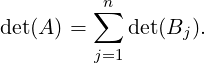
We now relate this definition of determinant with the one given in Definition 2.3.6.
Theorem 9.3.3. Let A be an n × n matrix. Then, det(A) = ∑
j=1n(-1)1+ja1j det A(1|j)
 ,
where recall that A(1|j) is the submatrix of A obtained by removing the 1st row and the jth
column.
,
where recall that A(1|j) is the submatrix of A obtained by removing the 1st row and the jth
column.
Proof. For 1 ≤ j ≤ n, define an n × n matrix Bj = 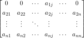 . Also, for each
matrix Bj, we define the n × n matrix Cj by
. Also, for each
matrix Bj, we define the n × n matrix Cj by
-
1.
- Cj[:,1] = Bj[:,j],
-
2.
- Cj[:,i] = Bj[:,i - 1], for 2 ≤ i ≤ j and
-
3.
- Cj[:,k] = Bj[:,k] for k ≥ j + 1.
Also, observe that Bj’s have been defined to satisfy B1[1,:] +  + Bn[1,:] = A[1,:] and
Bj[i,:] = A[i,:] for all i ≥ 2 and 1 ≤ j ≤ n. Thus, by Theorem 9.3.1.5,
+ Bn[1,:] = A[1,:] and
Bj[i,:] = A[i,:] for all i ≥ 2 and 1 ≤ j ≤ n. Thus, by Theorem 9.3.1.5,
 | (9.3.1) |

 DRAFT
DRAFT
Let us now compute det(Bj), for 1 ≤ j ≤ n. Note that Cj = E12E23 Ej-1,jBj, for 1 ≤ j ≤ n. Then,
by Theorem 9.3.1.3, we get det(Bj) = (-1)j-1 det(Cj). So, using Remark 9.3.2.2 and
Theorem 9.3.1.2 and Equation (9.3.1), we have
Ej-1,jBj, for 1 ≤ j ≤ n. Then,
by Theorem 9.3.1.3, we get det(Bj) = (-1)j-1 det(Cj). So, using Remark 9.3.2.2 and
Theorem 9.3.1.2 and Equation (9.3.1), we have
Thus, we have shown that the determinant defined in Definition
2.3.6 is valid. __
Theorem 9.4.1. Let V be a finite dimensional vector space over F and let W1 and W2 be two
subspaces of V. Then,
 | (9.4.1) |

 DRAFT
DRAFT
Proof. Since W1 ∩ W2 is a vector subspace of V , let  = {u1,…,ur} be a basis of W1 ∩ W2.
As, W1 ∩ W2 is a subspace of both W1 and W2, let us extend the basis to form a basis
1 = {u1,…,ur,v1,…,vs} of W1 and a basis 2 = {u1,…,ur,w1,…,wt} of W2.
= {u1,…,ur} be a basis of W1 ∩ W2.
As, W1 ∩ W2 is a subspace of both W1 and W2, let us extend the basis to form a basis
1 = {u1,…,ur,v1,…,vs} of W1 and a basis 2 = {u1,…,ur,w1,…,wt} of W2.
We now prove that  = {u1,…,ur,w1,…,ws,v1,v2,…,vt} is a basis of W1 + W2. To do this, we
show that
= {u1,…,ur,w1,…,ws,v1,v2,…,vt} is a basis of W1 + W2. To do this, we
show that
-
1.
- is linearly independent subset of V and
-
2.
- LS() = W1 + W2.
The second part can be easily verified. For the first part, consider the linear system
 | (9.4.2) |
in the variables αi’s, βj’s and γk’s. We re-write the system as

Then,
v =
-∑
i=1sγivi ∈ LS(
1) =
W1. Also,
v =
∑
j=1rαrur +
∑
k=1T βkwk. So,
v ∈ LS(
2) =
W2. Hence,
v ∈ W1 ∩ W2 and therefore, there exists scalars
δ1,…,δk such that
v =
∑
j=1rδjuj.

 DRAFT
DRAFT
Substituting this representation of v in Equation (9.4.2), we get

So,
using Exercise
3.4.16.
1,
αi -δi = 0, for 1
≤ i ≤ r and
βj = 0, for 1
≤ j ≤ t. Thus, the system (
9.4.2)
reduces to

which has
αi = 0 for 1
≤ i ≤ r and
γj = 0 for 1
≤ j ≤ s as the only solution. Hence, we see that the
linear system of Equations (
9.4.2) has no nonzero solution. Therefore, the set
is linearly
independent and the set
is indeed a basis of
W1 +
W2. We now count the vectors in the sets
,1,2 and
to get the required result. __
In this section, we prove the following result. A generalization of this result to complex vector space is
left as an exercise for the reader as it requires similar ideas.
Theorem 9.5.1. Let V be a real vector space. A norm ∥⋅∥ is induced by an inner product if and only
if, for all x,y ∈ V, the norm satisfies
Proof. Suppose that ∥⋅∥ is indeed induced by an inner product. Then, by Exercise 5.1.7.3 the result
follows.
So, let us assume that ∥⋅∥ satisfies the parallelogram law. So, we need to define an inner product.
We claim that the function f : V × V → ℝ defined by
 satisfies the required conditions for an inner product. So, let us proceed to do so.
-
- Step 1: Clearly, for each x ∈ V, f(x,0) = 0 and f(x,x) =
 ∥x + x∥2 = ∥x∥2. Thus,
f(x,x) ≥ 0. Further, f(x,x) = 0 if and only if x = 0.
∥x + x∥2 = ∥x∥2. Thus,
f(x,x) ≥ 0. Further, f(x,x) = 0 if and only if x = 0.
-
- Step 2: By definition f(x,y) = f(y,x) for all x,y ∈ V.
-
- Step 3: Now note that ∥x + y∥2 -∥x - y∥2 = 2
 . Or equivalently,
 | (9.5.2) |
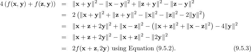
Thus, for x,y,z ∈ V, we have
Now, substituting z = 0 in Equation (9.5.3) and using Equation (9.5.2), we get
2f(x,y) = f(x,2y) and hence 4f(x + z,y) = 2f(x + z,2y) = 4 .
Thus,
.
Thus,
 | (9.5.4) |
-
- Step 4: Using Equation (9.5.4), f(x,y) = f(y,x) and the principle of mathematical induction, it
follows that nf(x,y) = f(nx,y), for all x,y ∈ V and n ∈ ℕ. Another application of
Equation (9.5.4) with f(0,y) = 0 implies that nf(x,y) = f(nx,y), for all x,y ∈ V and n ∈ ℤ.

 DRAFT
Also, for m≠0,
DRAFT
Also, for m≠0,
 Hence, we see that for all x,y ∈ V and a ∈ ℚ, f
 = af(x,y).
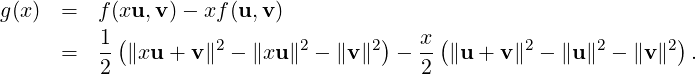
-
- Step 5: Fix u,v ∈ V and define a function g : ℝ → ℝ by Then, by previous step g(x) = 0, for all x ∈ ℚ. So, if g is a continuous function then continuity
implies g(x) = 0, for all x ∈ ℝ. Hence, f(xu,v) = xf(u,v), for all x ∈ ℝ.
Note that the second term of g(x) is a constant multiple of x and hence continuous. Using a
similar reason, it is enough to show that g1(x) = ∥xu + v∥, for certain fixed vectors u,v ∈ V, is
continuous. To do so, note that
 Thus,
Thus,  ∥x1u + v∥-∥x2u + v∥
 ≤∥(x1 - x2)u∥. Hence, taking the limit as x1 → x2, we get
limx1→x2∥x1u + v∥ = ∥x2u + v∥.
≤∥(x1 - x2)u∥. Hence, taking the limit as x1 → x2, we get
limx1→x2∥x1u + v∥ = ∥x2u + v∥.

 DRAFT
DRAFT
Thus, we have proved the continuity of g and hence the prove of the required result. _
The main aim of this subsection is to prove the continuous dependence of the zeros of a polynomial on
its coefficients and to recall Descartes’s rule of signs.
Definition 9.6.1. [Jordan Curves] A curve in ℂ is a continuous function f : [a,b] → ℂ, where
[a,b] ⊆ ℝ.
-
1.
- If the function f is one-one on [a,b) and also on (a,b], then it is called a simple curve.
-
2.
- If f(b) = f(a), then it is called a closed curve.
-
3.
- A closed simple curve is called a Jordan curve.
-
4.
- The derivative (integral) of a curve f = u+iv is defined component wise. If f′ is continuous
on [a,b], we say f is a
 1-curve (at end points we consider one sided derivatives and
continuity).
1-curve (at end points we consider one sided derivatives and
continuity).
-
5.
- A 1-curve on [a,b] is called a smooth curve, if f′ is never zero on (a,b).
-
6.
- A piecewise smooth curve is called a contour.
-
7.
- A positively oriented simple closed curve is called a simple closed curve such that while
traveling on it the interior of the curve always stays to the left. (Camille Jordan has proved
that such a curve always divides the plane into two connected regions, one of which is
called the bounded region and the other is called the unbounded region. The one which
is bounded is considered as the interior of the curve.)
We state the famous Rouche Theorem of complex analysis without proof.

 DRAFT
Theorem 9.6.2. [Rouche’s Theorem] Let C be a positively oriented simple closed contour.
Also, let f and g be two analytic functions on RC, the union of the interior of C and the curve
C itself. Assume also that |f(x)| > |g(x)|, for all x ∈ C. Then, f and f + g have the same
number of zeros in the interior of C.
DRAFT
Theorem 9.6.2. [Rouche’s Theorem] Let C be a positively oriented simple closed contour.
Also, let f and g be two analytic functions on RC, the union of the interior of C and the curve
C itself. Assume also that |f(x)| > |g(x)|, for all x ∈ C. Then, f and f + g have the same
number of zeros in the interior of C.
Corollary 9.6.3. [Alen Alexanderian, The University of Texas at Austin, USA.] Let
P(t) = tn + an-1tn-1 +  + a0 have distinct roots λ1,…,λm with multiplicities α1,…,αm,
respectively. Take any ϵ > 0 for which the balls Bϵ(λi) are disjoint. Then, there exists a δ > 0
such that the polynomial q(t) = tn + an-1′tn-1 +
+ a0 have distinct roots λ1,…,λm with multiplicities α1,…,αm,
respectively. Take any ϵ > 0 for which the balls Bϵ(λi) are disjoint. Then, there exists a δ > 0
such that the polynomial q(t) = tn + an-1′tn-1 +  + a0′ has exactly αi roots (counting with
multiplicities) in Bϵ(λi), whenever |aj - aj′| < δ.
+ a0′ has exactly αi roots (counting with
multiplicities) in Bϵ(λi), whenever |aj - aj′| < δ.
Proof. For an ϵ > 0 and 1 ≤ i ≤ m, let Ci = {z ∈ ℂ : |z - λi| = ϵ}. Now, for each i,1 ≤ i ≤ m, take
νi = minz∈Ci|p(z)|, ρi = maxz∈Ci[1 + |z| +  + |z|n-1] and choose δ > 0 such that ρiδ < νi. Then, for
a fixed j and z ∈ Cj, we have
+ |z|n-1] and choose δ > 0 such that ρiδ < νi. Then, for
a fixed j and z ∈ Cj, we have
 Hence, by Rouche’s theorem, p(z) and q(z) have the same number of zeros inside Cj, for
each j = 1,…,m. That is, the zeros of q(t) are within the ϵ-neighborhood of the zeros of
P(t). _
Hence, by Rouche’s theorem, p(z) and q(z) have the same number of zeros inside Cj, for
each j = 1,…,m. That is, the zeros of q(t) are within the ϵ-neighborhood of the zeros of
P(t). _
As a direct application, we obtain the following corollary.
Corollary 9.6.4. Eigenvalues of a matrix are continuous functions of its entries.
Proof. Follows from Corollary 9.6.3. _

 DRAFT
DRAFT
Remark 9.6.5.
-
1.
- [Sign changes in a polynomial] Let P(x) = ∑
0naixn-i be a real polynomial, with a0≠0.
Read the coefficient from the left a0,a1,…. We say the sign changes of ai occur at
m1 < m2 <
 < mk to mean that am1 is the first after a0 with sign opposite to a0; am2
is the first after am1 with sign opposite to am1; and so on.
< mk to mean that am1 is the first after a0 with sign opposite to a0; am2
is the first after am1 with sign opposite to am1; and so on.
-
2.
- [Descartes’ Rule of Signs] Let P(x) = ∑
0naixn-i be a real polynomial. Then, the
maximum number of positive roots of P(x) = 0 is the number of changes in sign of the
coefficients and that the maximum number of negative roots is the number of sign changes
in P(-x) = 0.
Proof. Assume that a0,a1, ,an has k > 0 sign changes. Let b > 0. Then, the coefficients
of (x - b)P(x) are
,an has k > 0 sign changes. Let b > 0. Then, the coefficients
of (x - b)P(x) are
 This list has at least k + 1 changes of signs. To see this, assume that a0 > 0 and an≠0.
Let the sign changes of ai occur at m1 < m2 <
This list has at least k + 1 changes of signs. To see this, assume that a0 > 0 and an≠0.
Let the sign changes of ai occur at m1 < m2 <  < mk. Then, setting
 we see that ci > 0 when i is even and ci < 0, when i is odd. That proves the claim.
Now, assume that P(x) = 0 has k positive roots b1,b2, ,bk. Then,

 DRAFT
DRAFT
 where Q(x) is a real polynomial. By the previous observation, the coefficients of (x -
bk)Q(x) has at least one change of signs, coefficients of (x-bk-1)(x-bk)Q(x) has at least
two, and so on. Thus coefficients of P(x) has at least k change of signs. The rest of the
proof is similar. _
where Q(x) is a real polynomial. By the previous observation, the coefficients of (x -
bk)Q(x) has at least one change of signs, coefficients of (x-bk-1)(x-bk)Q(x) has at least
two, and so on. Thus coefficients of P(x) has at least k change of signs. The rest of the
proof is similar. _
Let A ∈ Mn(ℂ) be a Hermitian matrix. Then, by Theorem 6.2.22, we know that all the eigenvalues of
A are real. So, we write λi(A) to mean the i-th smallest eigenvalue of A. That is, the i-th from the left
in the list λ1(A) ≤ λ2(A) ≤ ≤ λn(A).
Lemma 9.7.1. [Rayleigh-Ritz Ratio] Let A ∈ Mn(ℂ) be a Hermitian matrix. Then,
-
1.
- λ1(A)x*x ≤ x*Ax ≤ λn(A)x*x, for each x ∈ ℂn.
-
2.
- λ1(A) = minx≠0
 = min∥x∥=1x*Ax.
-
3.
- λn(A) = maxx≠0
 = max∥x∥=1x*Ax.
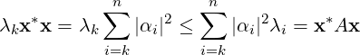
Proof. Proof of Part 1: By spectral theorem (see Theorem 6.2.22, there exists a unitary matrix U
such that A = UDU*, where D = diag(λ1(A),…,λn(A)) is a real diagonal matrix. Thus, the set
{U[:,1],…,U[:,n]} is a basis of ℂn. Hence, for each x ∈ ℂn, there exists _i’s (scalar) such that
x = ∑
αiU[:,i]. So, note that x*x = |αi|2 and

 DRAFT
DRAFT
 For
Part 2 and Part 3, take x = U[:,1] and x = U(:,n), respectively. _
For
Part 2 and Part 3, take x = U[:,1] and x = U(:,n), respectively. _
As an immediate corollary, we state the following result.
Corollary 9.7.2. Let A ∈ Mn(ℂ) be a Hermitian matrix and α =  . Then, A has an
eigenvalue in the interval (-∞,α] and has an eigenvalue in the interval [α,∞).
. Then, A has an
eigenvalue in the interval (-∞,α] and has an eigenvalue in the interval [α,∞).
We now generalize the second and third parts of Theorem 9.7.2.
Proposition 9.7.3. Let A ∈ Mn(ℂ) be a Hermitian matrix with A = UDU*, where U is a
unitary matrix and D is a diagonal matrix consisting of the eigenvalues λ1 ≤ λ2 ≤ ≤ λn.
Then, for any positive integer k,1 ≤ k ≤ n,
≤ λn.
Then, for any positive integer k,1 ≤ k ≤ n,
![λk = min x*Ax = max x *Ax.
x⊥U[:,∥x1]∥,.=..,1U[:,k-1] x⊥U[:∥,nx],∥..=.,U1[:,k+1]](LA2754x.png)
Proof. Let x ∈ ℂn such that x is orthogonal to U[,1],…,U[:,k - 1]. Then, we can write
x = ∑
i=knαiU[:,i], for some scalars αi’s. In that case,

 DRAFT
DRAFT
 and
the equality occurs for x = U[:,k]. Thus, the required result follows. _
and
the equality occurs for x = U[:,k]. Thus, the required result follows. _
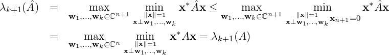
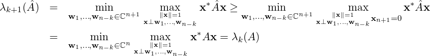
Theorem 9.7.4. [Courant-Fischer] Let A ∈ Mn(ℂ) be a Hermitian matrix with eigenvalues
λ1 ≤ λ2 ≤ ≤ λn. Then,

Proof. Let A = UDU*, where U is a unitary matrix and D = diag(λ1,…,λn). Now, choose a set of
k - 1 linearly independent vectors from ℂn, say S = {w1,…,wk-1}. Then, some of the eigenvectors
{U[:,1],…,U[:,k - 1]} may be an element of S⊥. Thus, using Proposition 9.7.3, we see
that
![λk = min x*Ax ≥ min x*Ax.
x⊥U[:∥,1x∥],=...1,U,[:,k-1] ∥xx∈∥=S1⊥](LA2760x.png) Hence, λk ≥ maxw1,…,wk-1 min ∥x∥=1
x⊥w1,…,wk-1 x*Ax, for each choice of k - 1 linearly independent vectors.
But, by Proposition 9.7.3, the equality holds for the linearly independent set {U[:,1],…,U[:,k - 1]}
Hence, λk ≥ maxw1,…,wk-1 min ∥x∥=1
x⊥w1,…,wk-1 x*Ax, for each choice of k - 1 linearly independent vectors.
But, by Proposition 9.7.3, the equality holds for the linearly independent set {U[:,1],…,U[:,k - 1]}

 DRAFT
which proves the first equality. A similar argument gives the second equality and hence the proof is
omitted. _
DRAFT
which proves the first equality. A similar argument gives the second equality and hence the proof is
omitted. _
Theorem 9.7.5. [Weyl Interlacing Theorem] Let A,B ∈ Mn(ℂ) be a Hermitian matrices.
Then, λk(A) + λ1(B) ≤ λk(A + B) ≤ λk(A) + λn(B). In particular, if B = P*P, for some
matrix P, then λk(A + B) ≥ λk(A). In particular, for z ∈ ℂn, λk(A + zz*) ≤ λk+1(A).
Proof. As A and B are Hermitian matrices, the matrix A + B is also Hermitian. Hence, by
Courant-Fischer theorem and Lemma 9.7.1.1,
and
If B = P*P, then λ1(B) = min∥x∥=1x*(P*P)x = min∥x∥=1∥Px∥2 ≥ 0. Thus,

 DRAFT
DRAFT

In particular, for z ∈ ℂn, we have
_
Proof. Note that
and _
As an immediate corollary, one has the following result.
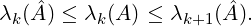
Corollary 9.7.7. [Inclusion principle] Let A ∈ Mn(ℂ) be a Hermitian matrix and r be a
positive integer with 1 ≤ r ≤ n. If Br×r is a principal submatrix of A then, λk(A) ≤ λk(B) ≤
λk+n-r(A).

 DRAFT
Theorem 9.7.8. [Poincare Separation Theorem] Let A ∈ Mn(ℂ) be a Hermitian matrix
and {u1,…,ur}⊆ ℂn be an orthonormal set for some positive integer r,1 ≤ r ≤ n. If further
B = [bij] is an r × r matrix with bij = ui*Auj,1 ≤ i,j ≤ r then, λk(A) ≤ λk(B) ≤ λk+n-r(A).
DRAFT
Theorem 9.7.8. [Poincare Separation Theorem] Let A ∈ Mn(ℂ) be a Hermitian matrix
and {u1,…,ur}⊆ ℂn be an orthonormal set for some positive integer r,1 ≤ r ≤ n. If further
B = [bij] is an r × r matrix with bij = ui*Auj,1 ≤ i,j ≤ r then, λk(A) ≤ λk(B) ≤ λk+n-r(A).
Proof. Let us extend the orthonormal set {u1,…,ur} to an orthonormal basis, say {u1,…,un} of ℂn
and write U = ![[ ]
u1 ⋅⋅⋅ un](LA2777x.png) . Then, B is a r × r principal submatrix of U*AU. Thus, by inclusion
principle, λk(U*AU) ≤ λk(B) ≤ λk+n-r(U*AU). But, we know that σ(U*AU) = σ(A) and hence the
required result follows. _
. Then, B is a r × r principal submatrix of U*AU. Thus, by inclusion
principle, λk(U*AU) ≤ λk(B) ≤ λk+n-r(U*AU). But, we know that σ(U*AU) = σ(A) and hence the
required result follows. _
The proof of the next result is left for the reader.
Corollary 9.7.9. Let A ∈ Mn(ℂ) be a Hermitian matrix and r be a positive integer with
1 ≤ r ≤ n. Then,

Proof. Let {x1,…,xn-k} be a basis of W⊥. Then,

 DRAFT
DRAFT

Now assume that x*Ax > 0 holds for each nonzero x ∈ W and that λn-k+1 = 0. Then, it follows
that min ∥x∥=1
x⊥x1,…,xn-k x*Ax = 0. Now, define f : ℂn → ℂ by f(x) = x*Ax.
Then, f is a continuous function and min∥x∥=1
x∈W f(x) = 0. Thus, f must attain its bound on the unit
sphere. That is, there exists y ∈ W with ∥y∥ = 1 such that y*Ay = 0, a contradiction. Thus, the
required result follows. _

 DRAFT
DRAFT

 DRAFT
DRAFT

 DRAFT
DRAFT


![[ ]
1 2
2 1](LA2658x.png) ,
det(
,
det(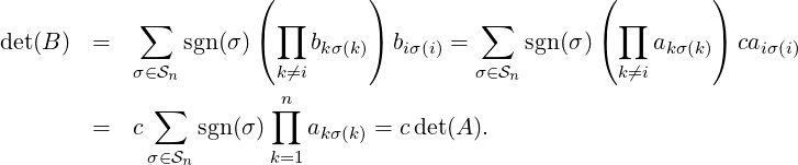


![λk(A + B) = max min x*(A + B )x
w1,...,wk-1 x⊥w ∥x∥,..=.,1w
1 k-1 *
≤ w1m,.a..x,wk-1 m∥xi∥n=1 [x Ax + λn(B )] = λk(A) + λn(B )
x⊥w1,...,wk-1](LA2763x.png)
![*
λk (A + B) = w1m,.a..,xwk-1 ∥mxi∥n=1 x (A + B )x
x⊥w1,...,wk- 1
≥ max min [x*Ax + λ1(B)] = λk(A)+ λ1 (B ).
w1,...,wk-1 x⊥w∥1x,∥..=.,1wk- 1](LA2764x.png)
![λk(A + zz*) = max min [x*Ax + |x*z|2]
w1,...,wk -1x⊥w∥1x∥,.=..1,wk-1
* * 2
≤ w1m,a...x,wk -1 ∥mxi∥n=1 [x Ax + |x z| ]
x⊥w1,...,wk-1,z
= max min x*Ax
w1,...,wk -1x⊥w∥1x,.∥..=,w1 ,z
k-1 *
≤ w1,...m,wakx-1,wk m∥ix∥n=1 x Ax = λk+1 (A ).
x⊥w1,...,wk-1,wk](LA2768x.png)
![[ ]
A y
y * a](LA2769x.png)


![[ ]
1 0
0 2](LA2780x.png)
