2.2.1 Antenna output and RF section
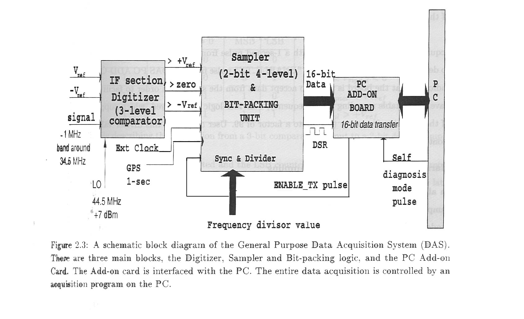
Antenna output, i.e. (E + W) sum voltage signal at 34.5 MHz, was fed to the DAS. The DAS consists of three parts. Please refer to figure 2.3 for the block diagram of the DAS. The first one is the "Digitizer Unit" which digitizes the input signal (IF) to three levels. The digitized information is fed to the second stage which is the "Bit-Packing Logic Unit" . This unit converts. the 2-bit data into a 16-bit parallel information compatible with a PC data bus. The 16-bit data are provided to the "DAS PC ADD-ON" card, which interfaces with the PC. These three units axe explained in detail in the following paragraphs.
2.2.2 Digitizer : IF section
The antenna signal at 34.5 MHz, with a bandwidth of ~2 MHz after an adequate amplification, is down-converted to an IF of 10 MHz using a Local Oscillator (LO) frequency of 44.5 MHz and a power level of +7 dBm. After an appropriate amplification, we filter this signal to obtain a 3 dB band width of 1-MHz around the central frequency of 10 MHz.
This unit further consists of three comparators which are realized using
high-speed operational amplifiers(NE521). Input signal is ac-coupled to
avoid any dc signal. This input signal level is compared to three reference
voltage levels, a positive "+Vref ", a negative ref "-Vref
",
and "Zero" level. Both +Vref and -Vref are generated
from the same source, so that a deviation in +Vref will e tracked
by deviations in the -Vref. Thus this unit generates three bits of information
(TTL logic levels) which tells the statistics and the nature of the input
signal. These bits are transferred on differential lines to the bit-packing
logic unit.
2.2.3 Sampler and bit-packing
All the units needed for the bit-packing logic are realized in a'Erasable Programmable Logic Device' (EPLD) chip (from Altera). To accomodate for any future changes in the logic only 70% to 80 of the logic cells of the EPLD are used.
A standard oscillator (of frequency fsin) is used as an input
clock for this block. The data acquisition can be synchronized with a 1-second
pulse from the Global Position System (GPS), if so desired. It is also
gated with the "ENABLE-TX' pulse from the DAS PC ADD-ON board which indicates
that the board is ready to accept data from the system. In order to facilitate
the user to have a selectable swnpling clock frequency, a divider logic
is employed, which supports a division of the incoming frequency (fsin)
upto a factor of 99. User can select this diviser value through the front
panel thumb wheel.
Harmonic sampling
In all our observations, we used fsin=21 MHz, and a division
factor of 10, which generates a sampling frequency (fs) of 2.1 MHz. The
fifth harmonic of this frequency falls at 10.5 MHz. This mode of sampling
is called Harmonic Sampling. It folds, among other bands, the band from
8.4 MHz to 10.5 MHz to a baseband from 0 to 1.05 MHz. We thus sample our
signal band between 9.45 MHz and 10.5 MHz, where the band is flipped to
fall b;tween 0 to 1.05 MHz. This method allows us to sample a band located
at an higher frequency with a low frequency sampler performing an implicit
down-conversion, a definite advantage from the design point of view.
3-bit comparator output to 2-bit sample conversion
A hardware for conversion from 3-bit comparator outputs to a 2-bit sample representation is realized using combinational logic. Please refer to Table 2.2 for this conversion. This block is also incorporated in the EPLD in order to support any other conversion/coding, if needed at a future date. Thus, for every cycle of the sampling clock we will get a 2-bit data sample.
It is helpful to pack a suitable number of these 2-bit samples to a
16-bit word so that data transfer to the PC can be optimised, since the
IESA bus used on a PC/AT supports a 16-bit data transfer. This, along with
a more efficient storage of data onto the PC, necessitates the bit-packing
logic. This block accepts two bits for each sampling clock and packs eight
successive samples to a 16-bit word. Before these bits axe passed to the
PC bus, they can be multiplexed with another 16-bit of locally generated
"marker" data. Such a marker word has its eight most significant bits (MSB)
as zeroes, with the least significant byte (LSB) acting as counter. For
every 4K-words of actual- data one such ,marker" is inserted and the
LSB counter is incremented. The LSB counter, thus keeps count(modulo 256)
of the 4K-word blocks of data transferred. These counts are later used
in checking for possible slips in the data acquisition.
2.2.4 PC interface card
This card functions as an interface between the high-speed data acquisition system and a PC. It is provided with two data storage buffers, which are First In First Out (FIFO) memory devices. The data are written in FIFO, and are accessed by the acquisition program.
The real contraints on the data acquisition rate comes from the disk access time of a PC, and the FIFO memory size. Since data rates of the order of 0.5 MB per second are expected, the disk access time should be <10ms for a FIFO of 8K. In the case of the disk access time being larger occasionally, it led to data slips in transfer. Such a loss in data can be checked using markers mentioned above. We discuss this in the section on data analysis. In our later set-up, which was used for the present observations, a new PC was used with a much faster disk, and a larger FIFO (32K) on the PC ADD-ON card.
2.2.5 Diagnostic mode
A self-diagnosis mode is incorporated to check the transmission of data
from the EPLD to the PC bus. In this diagnostics mode of operation, bit-backing
EPLD acts as a pair of 8-bit counters and the count is decremented / incremented
by appropriate signals from bit-packing logic. The counters are designed
such that one of the two 8-bit counters counts in "up" and the other in
the "down" modes. This will write lower bytes in the ascending order and
the upper byte in the descending order. This Pattern can be checked at
the data file. Any deviations can then be traced in the hardware.
2.3 Off-line processing
2-3.1 Data slip-check
As mentioned in section 2.2.3, for every 4096 words of data, we insert a 16-bit marker. The most significant bits (MSBs) are zero, and the least significant bits (LSBs) are used as a counter from zero to 255. The general probability that a data would mimick such a behavior is small (<=1 Part in 216), and that for such a data to arrive at the expected successive locations Of markers is negligible. An upcounter(with LSBs) is incremented after every 4096 words. In the event of data loss, the missing number of markers as well - the data words found between the recovered markers would identify and quantify such a data loss. Once a loss of marker from its expected location was encountered, the next Marker is identified by looking for a subsequent word which ha, its MS Byte equal to zero. Wherever a match occurred we read out the LSB of this word to check if a "sensible" value was found. From this marker onwards later markers Will be traced for data loss as described above.
We note separately a copy. of the first block of 4096 words of each
data file when we begin the slip-check. Once we identify a missing block
of data, we fill the "gap" with a pseudo-sequence obtained by randomizing
the samples from the "noted lst block". It should be noted that such data
loss was almost never encountered in our observations.
2.3.2 Digitizer level weightages
In the scheme of acquisition, the incoming signal voltages are sampled after digitization. Digital sampling is inherently a non-linear process: with a finite number of bits, 'quantization' noise will inevitably be added to the signal. The extreme case of 1-bit sampling, in which 'on' and 'off' values are assigned by comparing each sample to signal mean, yields the noisiest representation of the signal. The quantization we have chosen for DAS (2-bit, 4-level) is a significant improvement on 1-bit sampling, but still quite coarse. It was a compromise from the design Point of view: the motivation was to keep the data rate and data sizes to a manageable level while sampling with more than one bit. The coarse quantization will necessarily affect the observed pulse shapes and signal-to-noise ratios, but in statistically predictable ways.
The Primary concern in a coarsely quantized system is that of linearity, or in other words, the dynamic range: i.e., whether the response to a strong pulse feature is the same as to a weaker component. Another potential problem, a result of the dedispersion convolution, is the possible appearance of dips to either side of the pulse peaks. This problem is most prominent in the case of 1-bit sampling, but similar problem may easily occur in 2-bit quantized profiles. We have determined that the linearity is optimized by correctly choosing the spacing of the quantization levels or decision thresholds relative to the root-mean-square (rms) voltage of the incoming signal.
Consider the case of 2-bit quantization, with decision thresholds -Vref, 0 and +Vref and the decoded output levels spaced to be -n, -1, 1 and +n, where n is not necessarily an integer. We have found, using simulations, that |Vref| ~ 1.0 Vrms and n ~ 3.8 are optimal values for these parameters, as compared to using |Vref|= 1.0 and n = 3 (Thompson, Moran, Swenson, 1986). In our simulations, we start with generating a series of random numbers (RN) with a mean zero and standard deviation of 1. We digitize the random numbers, sample-by-sample, with particular symmetric thresholds (± Vref).he digitized value was assigned a weight (D) of +LOW or +HIGH if the random number was smaller than +Vref or larger respectively. Similarly, a weight of -LOW or -HIGH was assigned if the value was higher than -Vref or lower respectively. For various values of Vref, LOW and HIGH, we compute a simple chi-square quantity, which measures the departure of the digitized numbers from analog numbers, which was defined by . We now track this value of chi-square as a function +Vref, LOW and HIGH. For a more faithful reconstruction, this value would be minimized. The results, even though obtained with random numbers as input, are valid for our data since pulsar signals are weak in the decameter band.
Stairs (Stairs, 1998) has dealt with this issue in detail, and our values match with their optimum parameters well. It was shown, that setting |Vref|= 1.4Vrms and n = 4 best preserves the pulse shape while making the final signal-to-noise ratio roughly 0.82 of the analog value, as compared to the 0.66 fraction expected from using |Vref|= 1.0 and n = 3 (Thompson, Moran, Swenson, 1986).
In practice, on-source response of GEETEE is modulated by beam-flips
over timescales of 40 sec(d) s (section 2.1.2)
and there are systematic changes in the system gain of the order of 2dB.
A dynamic setting with |Vref|= 1.4Vrms was not possible. Therefore,
we estimated the at quantized Vrms at the beginning of the data
acquisition by computing histograms of the incoming data using n = 3. We
then adjusted the input attenuation until the |Vref| is about
Vrms. This arrangement made it possible for the digitization
thresholds to remain close to the optimum value in entire acquisition.
2.3.3 An Effective Spectrometer
Raw spectrum, with a desired number of channels (nchan), is computed from the digitized voltage samples in overlapping blocks of 2nchan by means of Fourier Transform. The maximum time resolution in each channel then is the inverse of the channel width delta_nuchan. If so desired, the output is obtained by adding specified number of consecutive spectra (m) together. In this case the time resolution is (m.nchan) µ-s.
This way, we construct the output of an effective spectrometer output
with nchan spectral channels, as a function of time, with
desired time-resolution ( referred as taudelta_nu
).
Optimum resolution consideration
We now have data matrix of nchan channels with desired time
resolution (taudelta_nu
). If we know the amount of dispersion caused by the interstellar medium,
we can correct the differential dispersion delay within our band relative
to some reference channel (section 1.3.1). Due to this procedure,any dispersion
delay spread within a single channel remains, however, uncompensated and
thus effects another time constant (taud).
Other contribution to the temporal smearing arises due to the interstellar
scattering (tausc).
The effective time resolution can, therefore, be written as,
where, taud = 8300 DM delta_nu/(nchan nu03)s, taudelta_nu ~ (nchan/delta_nu) µ-s, and delta_nu & nu0 are bandwidth & central frequency of observation (in units of MHz) respectively.
We choose nchan so that taud
= taudelta_nu, for an
optimum resolution/smoothing (Deshpande, 1989;
gzipped psfile).
This condition leads us to an optimum
number of channels for dedispersion in the present case as
nchan~ 450 DM1/2.
Interferrence detection and excision
Shown in figures 2.4 and 2.5 are the raw time series data and raw spectrum, where dispersion correction has not been applied. Such plots give information on the quality of the data and presence of any interference which is necessarily "local" (so, undispersed).
The raw time series essentially shows the variations of the system gain with time. The jumps in the power level, most notably close to 135 and 205 seconds, are due to gain changes corresponding to beam-flips during source tracking (using discrete beam directions). The time duration between two successive beam-flips is 40sec(dec) seconds, where dec is the source declination. Any large fluctuations (say, > 10 rms) over a time-duration much shorter than the transit time across the beam-width of the array in the E-W, which corresponds to about 1.5 minutes at dec= 0,are due to interference.
The interference is either narrow-band, in which case it is seen as sharp peaks in the spectrum (figure 2.5). Such an interferrence consists of broader spike-like recurring variations over a longer duration in the time-doniain, and may occur due to terrestrial radio broadcast signals. Sharp peaks in the time domain, typically due to electric lightening or due to faulty electric gadgets in the near viscinity of the antenna, on the other hand, have much broader spread in the raw frequency spectrum.
Different kinds of interference were treated after visual inspection of the raw time series and its radio frequency spectrum. Narrow- and broad-band interference are apparent in the spectra as large changes in the fluctuation of the channel power relative to the neighbouring channels. Channels with fluctuations typically more than 5 times of fluctuations in the nearby channels were 'flagged' for rejection from the later analysis.
By summing the spectral contribution across the spectrum, after rejecting the flagged inter-ference channels, we obtain a time sequence similar to the one shown in the figure 2.4. We manually deleted parts of the time series containing sharp -peaks (typically > 10 rms) or interference over a broader duration.
Information about the raw time sequence and the spectrum is stored in
an additional data file, called 'config' file, which is accessed in the
further analysis. The steps of interference excision are flexible. In case
a major portion of data has a continuous patch of large interference, spectrum
is recomputed from the raw data (going back one stage in the analysis procedure)
excluding that part of the raw data. Further steps in analysis now depend
upon the intended study of the pulsar.
2.3.4 Channel-wise folded proflles
With the knowledge of the spin period of the pulsar, we fold the time
series in each channels at that period. Such folded pulse profiles can
be viewed across our band. The pulse peak shows expected dispersion delay
across the band, as shown in the figure 2.6. This matrix of data, intensity
as a function of channel number and phase bin, can be utilized in various
ways.
Average folded profile
We can now estimate the average profile of the pulsar from the above-mentioned matrix of data. Suitable delays are applied to the longitude time series in each channel compensating for the differential dispersion delay across the and. Folded pulse profiles from all the channels are summed ('channel-collapse') to obtain a dispersion-corrected pulse profile (incoherent dedispersion)