Blasius Profile
The Blasius profile is a solution of the Navier Stokes equations for a flow close to a semi-infinite flat plate. Firstly, by assuming that the flat plate is infinitely long along the spanwise direction, we can ignore variations along one-dimension entirely. Secondly, the flow is assumed steady, so that derivatives with respect to time are neglected as well. This allows us to start off with the 2D steady-state Navier-Stokes equations:
$$ \frac{\partial u}{\partial x} + \frac{\partial v}{\partial y} = 0 $$ $$ u\frac{\partial u}{\partial x} + v\frac{\partial u}{\partial y} = -\frac{\partial p}{\partial x} + \nu\left(\frac{\partial^2 u}{\partial x^2} + \frac{\partial^2 u}{\partial y^2}\right) $$ $$ u\frac{\partial v}{\partial x} + v\frac{\partial v}{\partial y} = -\frac{\partial p}{\partial y} + \nu\left(\frac{\partial^2 v}{\partial x^2} + \frac{\partial^2 v}{\partial y^2}\right) $$We use a scaling argument to assert that \(v \ll u\) and that variations of quantities along the \(x\) direction are much smaller than those along the \(y\) direction. Moreover, we assume that the pressure gradient along the \(x\) direction is 0. This allows us to reduce the above equations to the following equation for \(u\):
$$ u\frac{\partial u}{\partial x} + v\frac{\partial u}{\partial y} = \nu\frac{\partial^2 u}{\partial y^2} $$Let the free-stream velocity be \(U\) and let \(\delta\) be the boundary layer thickness. Blasius established that \(\delta(x) \propto \sqrt{\nu x/U}\), and normalized the \(y\) coordinate as \(\eta(x) = y/\delta(x)\). Subsequently we introduce a normalized stream-function \(\psi\) in terms of \(\eta\) as \(\psi = \sqrt{\nu U x} f(\eta)\). Keeping in mind that \(u = \partial\psi/\partial y\) and that \(v = -\partial\psi/\partial x\), and with a bit of algebra, the above equation for \(u\) will reduce to the Blasius ODE as
$$ 2f''' + f''f = 0, \qquad \qquad f(0) = 0, \qquad \qquad f'(0) = 0, \qquad \qquad f'(\infty) = 1. $$When solving an ODE, there are two ways we can go about with it. If we know the initial values of all the variables, we can start from these values and march forward in \(\eta\). Such problems are called Initial Value Problems (IVP). In other cases, we know the values of the variables at the boundaries of the domain, in which case we usually solve the equations iteratively. Such problems are Boundary Value Problems (BVP). Here we have a BVP, but one of the boundaries is at \(\infty\), and we use a method called shooting method to solve it.
Now solving the Blasius ODE with shooting method using Python is the fun part. By introducing two new variables, \(g\) and \(h\), as below, we first obtain a set of three ODEs.
$$ g = f', \qquad \qquad h = f'' $$So the derivatives of these two new variables will be:
$$ g' = f'' = h, \qquad \qquad h' = f''' = -\frac{f''f}{2} = -\frac{hf}{2}. $$We now have a set of ODEs which can be solved simultaneously as below:
$$ \frac{\partial}{\partial \eta} \begin{bmatrix} f \\ g \\ h \end{bmatrix} = \begin{bmatrix} g \\ h \\ -hf/2 \end{bmatrix} $$In Python, this equation can be written as a simple function as below:
    def blasiusEqn(eta, y):
        f, g, h = y
        return g, h, -h*f/2
This is an example of a non-autonomous ODE, since the variable of differentiation, \(\eta\) does not appear in the equations.
However, for the ODE solving functions of SciPy module to be used later, the variable of differentiation must also be defined as an argument of the function.
Hence, eta has also been included as a parameter, although it is not used anywhere in the function.
Moreover, the variables \(f\), \(g\) and \(h\) have been packed together into a single vector y, for convenience.
Now we need to integrate the ODE using an integrating function of SciPy.
For this, we will use the RK45 function from scipy.integrate.
We need to pass the initial value of \(\eta\) (which is 0), along with the initial values of \(f\), \(g\) and \(h\).
Now we know the initial values of \(f\) and \(g\), but not that of \(h\).
But what if we guessed an initial value for \(h\)?
To do that, we will first represent these initial values as f0, g0 and h0 in the code.
Then we write a function that already knows the values of f0 and g0 to be 0, but accepts a guessed value of h0 as an argument.
It then solves the ODE using this guessed value for a reasonably large number of steps
(since we can't compute all the way up to infinity, we are content with using a sufficiently large value as an approximation).
After solving, we check the value of g (which is y[1] since we packed f, g and h
into a single variable y) and see how close it is to the expected value of 1 at infinity.
    import scipy.integrate as integrate

    def findh0(h0):
        f0, g0 = 0, 0
        initVals = np.array([f0, g0, h0], dtype=object)
        res = integrate.RK45(blasiusEqn, 0, initVals, 100)
        for i in range(100):
            res.step()

        return 1 - res.y[1]
Note that the function subtracts 1 from the value of res.y[1] (aka \(f'(\infty)\)) so that with the correct value of h0 when \(f'(\infty) = g = 1\), the code will output 0.
Let us now test the above function by passing a series of possible values for h0, that is, \(f''(0)\).
We will pass 9 values from 0.1 to 0.9, at increments of 0.1 in a for loop as below:
    for i in range(1, 10):
        print(i/10, findh0(i/10))
When we run the above code, we get the following output:
    0.1 0.5506351233427067
    0.2 0.2866459873213928
    0.3 0.06532864818390183
    0.4 -0.13224447107866233
    0.5 -0.3138520833820062
    0.6 -0.4836714704127618
    0.7 -0.6442724624772207
    0.8 -0.7973778017977666
    0.9 -0.9442182127881427
We see that somewhere between 0.3 and 0.4, the output of the function changes sign from positive to negative!
This is close to the expected value of 0.332, and we must now try to get this value using a non-linear solver.
We will employ the next useful SciPy function for our task - fsolve from scipy.optimize.
This makes our task so absurdly simple, that we only need to pass the function, findh0,
and an initial guessed value, for which we choose 0.3, since we just found that to be pretty close to the root of the function.
Thus we find the expected value with just a one-line code.
    import scipy.optimize as optimize

    h0 = optimize.fsolve(findh0, 0.3)
    print(h0[0])
This will very nicely print the expected value of h0 as 0.332 which is indeed the expected value.
Putting it all together, we can now solve the Blasius equation and plot the resulting velocity profile with a short Python code:
    import matplotlib.pyplot as plt

    def blasius():
        f0, g0 = 0, 0
        h0 = optimize.fsolve(findh0, 0.3)
        initVals = np.array([f0, g0, h0], dtype=object)
        res = integrate.solve_ivp(blasiusEqn, (0, 10), initVals, max_step=0.01)

        eta = res.t
        g = res.y[1]

        # Now plot the profile
        fig = plt.figure(figsize=(7.5, 9))
        ax = fig.add_subplot(1, 1, 1)

        ax.plot(g, eta, linewidth=3, color='r')

        ax.set_xlim(0, 1.2)
        ax.set_ylim(0, 10)
        ax.set_xlabel(r"$f'$", fontsize=35)
        ax.set_ylabel(r"$\eta$", fontsize=35)
        ax.tick_params(axis='both', which='major', labelsize=30)

        plt.tight_layout()
        plt.show()

    blasius()
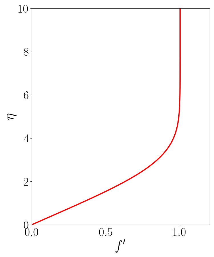
Two things to note in the above code are that (a) we use the function solve_ivp instead of RK45 because it gives finer control
on the spacing of points in the final result so that we get a neat-looking plot, and (b) we are actually plotting \(g = f'(\eta)\) because \(f\) is merely
the non-dimensional stream-function. The actual velocity profile is given by its derivative.
Finally we see Blasius profile in the flesh: