Tangent-Hyperbolic Grid
The finite-difference code SARAS uses non-uniform grids to increase resolution near the walls. To generate non-uniform spacing, a tangent-hyperbolic function is used:
$$ x = \frac{L}{2}\left[1 - \frac{\tanh{[\beta(1 - 2\xi)]}}{\tanh{\beta}}\right] $$Here, \(\xi\) varies uniformly from \(0\) to \(1\), but \(x\) varies non-uniformly from \(0\) to \(L\). Below is a set of 5 non-uniform grids spanning a domain of \(L = 2.0\), with \(\beta\) ranging from \(0.8\) to \(2.0\). The grid is very finely spaced at either ends of the domain, and coarse around the center, at \(\xi = 0.5\). Such grids are useful for simulating internal flows like channel flows, where the domain is bounded by no-slip walls at both ends.
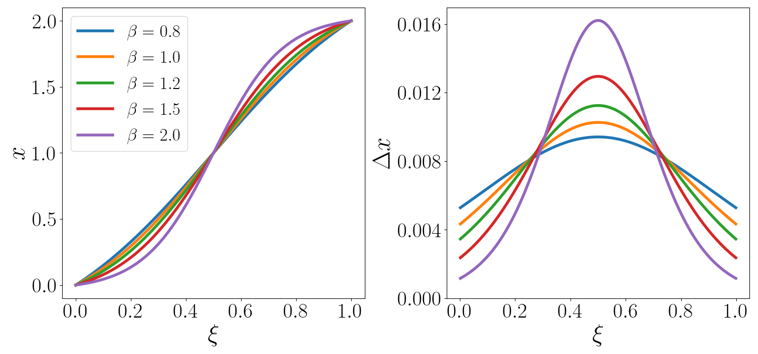
As the stretching parameter \(\beta\) increases, the non-uniformity of the grid also increases. For very high values of \(\beta\), the grid stretches so widely that the lowest spacing is \(\Delta x_{min} = 0.0012\), while the maximum spacing is \(\Delta x_{max} = 0.016\). With orthogonal grids in 2D or 3D domains, such high stretching can produce cells of skewness greater than 10. This can introduce a great degree of inaccuracy in some finite-difference codes. It is safe to keep \(\beta\) less than 1.8 in such cases.
It is also possible to have grids that are fine at one end of the domain and coarse at the other end. Such grids are useful for simulating external flows, where the grid has to be fine near the surface of a body (like an airfoil), but can be less resolved farther away into the flow field. A slightly modified form of the equation is used to achieve this:
$$ x = L\left[1 - \frac{\tanh{[\beta(1 - \xi)]}}{\tanh{\beta}}\right] $$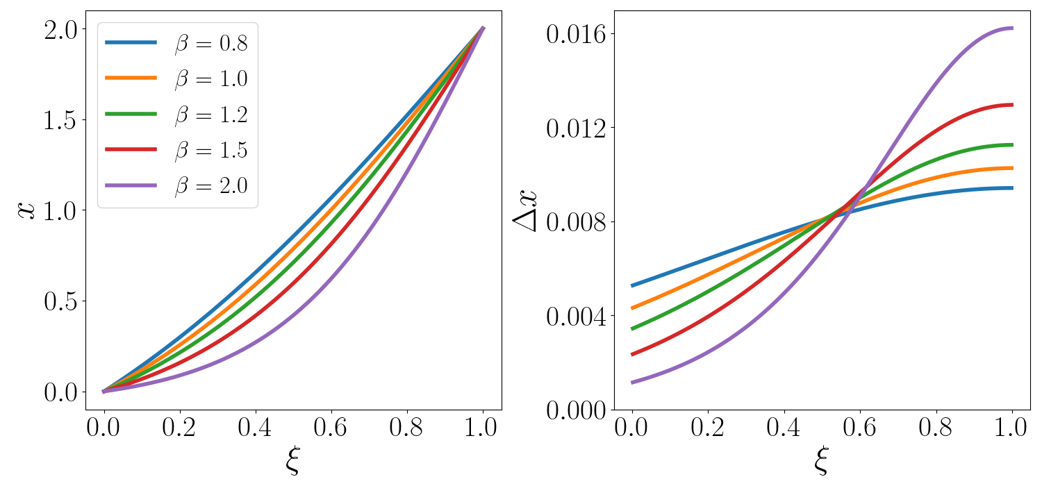
Finally, all derivatives are calculated with respect to \(\xi\) on the uniform grid, and transformed to the non-uniform grid using chain rule:
$$ \frac{\partial f}{\partial x} = \frac{\partial \xi}{\partial x}\frac{\partial f}{\partial \xi} $$ $$ \frac{\partial^2 f}{\partial x^2} = \frac{\partial^2 \xi}{\partial x^2}\frac{\partial f}{\partial \xi} + \left(\frac{\partial \xi}{\partial x}\right)^2\frac{\partial^2 f}{\partial \xi^2} $$The above formulae apply to simple orthogonal coordinate systems. With curvilinear coordinates, more terms will appear in the equation. Just as \(\xi\) corresponds to the transformed grid along \(x\), we have \(\eta\) and \(\zeta\) as the corresponding coordinates for \(y\) and \(z\) respectively. Then we will have contributions from derivatives with respect to these coordinates as well in the final equation for derivatives in physical plane.