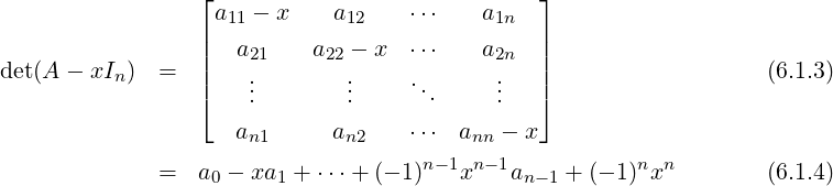
In this chapter, every matrix is an element of Mn(ℂ) and x = (x1,…,xn)T ∈ ℂn, for some n ∈ ℕ. We
start with a few examples to motivate this chapter.
Example 6.1.1.
-
1.
- Let A =
![[ ]
1 2
2 1](LA1766x.png) , B =
, B = ![[ ]
9 - 2
- 2 6](LA1767x.png) and x =
and x = ![[ ]
x
y](LA1768x.png) .
.
-
(a)
- Then A magnifies the nonzero vector
![[ ]
1
1](LA1769x.png) three times as A
three times as A![[ ]
1
1](LA1770x.png) = 3
= 3![[ ]
1
1](LA1771x.png) and behaves
by changing the direction of
and behaves
by changing the direction of ![[ ]
1
- 1](LA1772x.png) as A
as A![[ ]
1
- 1](LA1773x.png) = -1
= -1![[ ]
1
- 1](LA1774x.png) . Further, the vectors
. Further, the vectors ![[ ]
1
1](LA1775x.png) and
and ![[ ]
1
- 1](LA1776x.png) are orthogonal.
are orthogonal.
-
(b)
- B magnifies both the vectors
![[ ]
1
2](LA1777x.png) and
and ![[ ]
- 2
1](LA1778x.png) as B
as B![[ ]
1
2](LA1779x.png) = 5
= 5![[ ]
1
2](LA1780x.png) and B
and B![[ ]
2
- 1](LA1781x.png) =
10
=
10![[ ]
2
- 1](LA1782x.png) . Here again, the vectors
. Here again, the vectors ![[ ]
1
2](LA1783x.png) and
and ![[ ]
2
- 1](LA1784x.png) are orthogonal.
are orthogonal.
-
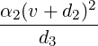
(c)
- xT Ax = 3
 -
- . Here, the displacements occur along perpendicular
lines x + y = 0 and x - y = 0, where x + y = (x,y)
. Here, the displacements occur along perpendicular
lines x + y = 0 and x - y = 0, where x + y = (x,y)![[ ]
1
1](LA1787x.png) and x - y = (x,y)
and x - y = (x,y)![[ ]
1
- 1](LA1788x.png) .
.
Whereas, xT Bx = 5 + 10
+ 10 . Here also the maximum/minimum
displacements occur along the orthogonal lines x + 2y = 0 and 2x - y = 0, where
x + 2y = (x,y)
. Here also the maximum/minimum
displacements occur along the orthogonal lines x + 2y = 0 and 2x - y = 0, where
x + 2y = (x,y)![[ ]
1
2](LA1791x.png) and 2x - y = (x,y)
and 2x - y = (x,y)![[ ]
2
- 1](LA1792x.png) .
.
-
(d)
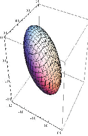
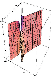
- the curve xT Ax = 10 represents a hyperbola, where as the curve xT Bx = 10
represents an ellipse (see Figure 6.1 drawn using the package “Sagemath”).
-
2.
- Let C =
![[ ]
1 2
1 3](LA1795x.png) , a non-symmetric matrix. Then, does there exist a nonzero x ∈ ℂ2 which gets
magnified by C?
, a non-symmetric matrix. Then, does there exist a nonzero x ∈ ℂ2 which gets
magnified by C?
So, we need x≠0 and α ∈ ℂ such that Cx = αx ⇔ [αI2 -C]x = 0. As x≠0, [αI2 -C]x = 0 has a
solution if and only if det[αI - A] = 0. But,
![([ ] )
α- 1 - 2
det[αI - A] = det = α2 - 4α + 1.
- 1 α - 3](LA1796x.png) So, α = 2 ±
So, α = 2 ± . For α = 2 +
  , verify that the x≠0 that satisfies
 ![[ √-- ]
1 + 3 √ --- 2
- 1 3 - 1](LA1799x.png) x = 0
equals x =
x = 0
equals x = ![[ √3-- 1]
1](LA1800x.png) . Similarly, for α = 2 -
. Similarly, for α = 2 - , the vector x =
 ![[ √3-+ 1]
- 1](LA1802x.png) satisfies
satisfies
![[ ]
1 - √3- - 2
√ --
- 1 - 3- 1](LA1803x.png) x = 0. In this example,
x = 0. In this example,
-
(a)
- we still have magnifications in the directions
![[√ -- ]
3- 1
1](LA1804x.png) and
and ![[√ -- ]
3+ 1
- 1](LA1805x.png) .
.
-
(b)
- the maximum/minimum displacements do not occur along the lines (
 -1)x+y = 0
and (
-1)x+y = 0
and ( + 1)x - y = 0 (see the third curve in Figure 6.1).
-
(c)
- the lines (
 - 1)x + y = 0 and (
 + 1)x - y = 0 are not orthogonal.
-
3.
- Let A be a real symmetric matrix. Consider the following problem:

 DRAFT
DRAFT
 To solve this, consider the Lagrangian
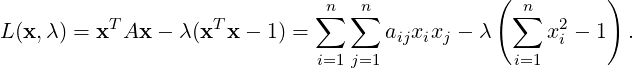 Partially differentiating L(x,λ) with respect to xi for 1 ≤ i ≤ n, we get
 | = 2a11x1 + 2a12x2 +  + 2a1nxn - 2λx1, + 2a1nxn - 2λx1, | |
|
 | =  | |
|
 | = 2an1x1 + 2an2x2 +  + 2annxn - 2λxn. + 2annxn - 2λxn. | | |
Therefore, to get the points of extremum, we solve for
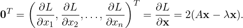 Thus, to solve the extremal problem, we need λ ∈ ℝ, x ∈ ℝn such that x≠0 and
Ax = λx.
Thus, to solve the extremal problem, we need λ ∈ ℝ, x ∈ ℝn such that x≠0 and
Ax = λx.
We observe the following about the matrices A,B and C that appear in Example 6.1.1.
-
1.
- det(A) = -3 = 3 ×-1, det(B) = 50 = 5 × 10 and det(C) = 1 = (2 +
 ) × (2 -
 ).
).
-
2.
- tr(A) = 2 = 3 - 1, tr(B) = 15 = 5 + 10 and det(C) = 4 = (2 +
 ) + (2 -
 ).
).
-
3.
- The sets
![{ [ ] [ ]}
1 , 1
1 - 1](LA1827x.png) ,
, ![{[ ] [ ]}
1 , 2
2 - 1](LA1828x.png) and
and ![{[ √-- ] [√ -- ]}
3 - 1 , 3 + 1
1 - 1](LA1829x.png) are linearly
independent.
are linearly
independent.
-
4.
- If v1 =
![[ ]
1
1](LA1830x.png) and v2 =
and v2 = ![[ ]
1
- 1](LA1831x.png) and S =
and S = ![[v1,v2 ]](LA1832x.png) then
then
-
(a)
- AS =
![[Av1,Av2 ]](LA1833x.png) =
= ![[3v1, - v2]](LA1834x.png) = S
= S![[ ]
3 0
0 - 1](LA1835x.png) ⇔ S-1AS =
⇔ S-1AS = ![[ ]
3 0
0 - 1](LA1836x.png) = diag(3,-1).
= diag(3,-1).
-
(b)
- Let u1 =
 v1 and u2 =
  v2. Then, u1 and u2 are orthonormal unit vectors, i.e.,
if U =
v2. Then, u1 and u2 are orthonormal unit vectors, i.e.,
if U = ![[u ,u ]
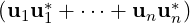
1 2](LA1839x.png) then I = UU* = u1u1* + u2u2* and A = 3u1u1*- u2u2*.
then I = UU* = u1u1* + u2u2* and A = 3u1u1*- u2u2*.
-
5.
- If v1 =
![[ ]
1
2](LA1840x.png) and v2 =
and v2 = ![[ ]
2
- 1](LA1841x.png) and S =
and S = ![[v1,v2 ]](LA1842x.png) then
then
-
(a)
- AS =
![[Av1,Av2 ]](LA1843x.png) =
= ![[5v1, 10v2]](LA1844x.png) = S
= S![[ ]
5 0
0 10](LA1845x.png) ⇔ S-1AS =
⇔ S-1AS = ![[ ]
5 0
0 10](LA1846x.png) = diag(3,-1).
= diag(3,-1).
-
(b)
- Let u1 =
 v1 and u2 =
  v2. Then, u1 and u2 are orthonormal unit vectors, i.e.,
if U =
v2. Then, u1 and u2 are orthonormal unit vectors, i.e.,
if U = ![[u1,u2 ]](LA1849x.png) then I = UU* = u1u1* + u2u2* and A = 5u1u1* + 10u2u2*.
then I = UU* = u1u1* + u2u2* and A = 5u1u1* + 10u2u2*.
-
6.
- If v1 =
![[ ]
√3-- 1
1](LA1850x.png) and v2 =
and v2 = ![[ ]
√3-+ 1
- 1](LA1851x.png) and S =
and S = ![[v1, v2]](LA1852x.png) then
then

 DRAFT
DRAFT
![[ ]
2+ √3- 0 √-- √ --
S -1CS = √ --= diag(2+ 3,2 - 3).
0 2 - 3](LA1853x.png)
Thus, we see that given A ∈ Mn(ℂ), the number λ ∈ ℂ and x ∈ ℂn,x≠0 satisfying Ax = λx have
certain nice properties. For example, there exists a basis of ℂ2 in which the matrices A,B and C
behave like diagonal matrices. To understand the ideas better, we start with the following
definitions.
Definition 6.1.2. [Eigenvalues, Eigenvectors and Eigenspace] Let A ∈ Mn(ℂ). Then,
-
1.
- the equation
 | (6.1.1) |
is called the eigen-condition.
-
2.
- an α ∈ ℂ is called a characteristic value/root or eigenvalue or latent root of A if there
exists x≠0 satisfying Ax = αx.
-
3.
- an x≠0 satisfying Equation (6.1.1) is called a characteristic vector or eigenvector or
invariant/latent vector of A corresponding to λ.
-
4.
- the tuple (α,x) with x≠0 and Ax = αx is called an eigen-pair or characteristic-pair.
-
5.
- for an eigenvalue α ∈ ℂ, Null(A - αI) = {x ∈ ℝn|Ax = αx} is called the eigenspace or
characteristic vector space of A corresponding to α.

 DRAFT
DRAFT
Theorem 6.1.3. Let A ∈ Mn(ℂ) and α ∈ ℂ. Then, the following statements are equivalent.
-
1.
- α is an eigenvalue of A.
-
2.
- det(A - αIn) = 0.
Proof. We know that α is an eigenvalue of A if any only if the system (A-αIn)x = 0 has a non-trivial
solution. By Theorem 2.2.40 this holds if and only if det(A - αI) = 0. _
Definition 6.1.4. [Characteristic Polynomial / Equation, Spectrum and Spectral Radius] Let
A ∈ Mn(ℂ). Then,
-
1.
- det(A-λI) is a polynomial of degree n in λ and is called the characteristic polynomial
of A, denoted PA(λ), or in short P(λ).
-
2.
- the equation PA(λ) = 0 is called the characteristic equation of A.
-
3.
- The multi-set (collection with multiplicities) {α ∈ ℂ : PA(α) = 0} is called the spectrum
of A, denoted σ(A). Hence, σ(A) contains all the eigenvalues of A.
-
4.
- The Spectral Radius, denoted ρ(A) of A ∈ Mn(ℂ), equals max{|α| : α ∈ σ(A)}.
We thus observe the following.
Remark 6.1.5. Let A ∈ Mn(ℂ).

 DRAFT
DRAFT
-
1.
- Then, A is singular if and only if 0 ∈ σ(A).
-
2.
- Further, if α ∈ σ(A) then the following statements hold.
-
(a)
- {0} ⊊ Null(A - αI). Therefore, if Rank(A - αI) = r then r < n. Hence, by
Theorem 2.2.40, the system (A-αI)x = 0 has n-r linearly independent solutions.
-
(b)
- x ∈ Null(A - αI) if and only if cx ∈ Null(A - αI), for c≠0.
-
(c)
- If x1,…,xr ∈ Null(A - αI) are linearly independent then ∑
i=1rcixi ∈ Null(A -
αI), for all ci ∈ ℂ. Hence, if S is a collection of eigenvectors then, we necessarily
want the set S to be linearly independent.
-
(d)
- Thus, an eigenvector v of A is in some sense a line ℓ = Span({v}) that passes
through 0 and v and has the property that the image of ℓ is either ℓ itself or 0.
-
3.
- Since the eigenvalues of A are roots of the characteristic equation, A has exactly n eigenvalues,
including multiplicities.
-
4.
- If the entries of A are real and α ∈ σ(A) is also real then the corresponding eigenvector has real
entries.
-
5.
- Further, if (α,x) is an eigenpair for A and f(A) = b0I + b1A +
 + bkAk is a polynomial in A
then (f(α),x) is an eigenpair for f(A).
+ bkAk is a polynomial in A
then (f(α),x) is an eigenpair for f(A).
Almost all books in mathematics differentiate between characteristic value and eigenvalue as the
ideas change when one moves from complex numbers to any other scalar field. We give the following
example for clarity.
Remark 6.1.6. Let A ∈ M2(F). Then, A induces a map T ∈ (F2) defined by T(x) = Ax, for all
x ∈ F2. We use this idea to understand the difference.
(F2) defined by T(x) = Ax, for all
x ∈ F2. We use this idea to understand the difference.
-
1.
- Let A =
![[ ]
0 1
- 1 0](LA1862x.png) . Then, pA(λ) = λ2 + 1. So, ±i are the roots of P(λ) = 0 in ℂ.
Hence,
. Then, pA(λ) = λ2 + 1. So, ±i are the roots of P(λ) = 0 in ℂ.
Hence,

 DRAFT
DRAFT
-
(a)
- A has (i,(1,i)T ) and (-i,(i,1)T ) as eigen-pairs or characteristic-pairs.
-
(b)
- A has no characteristic value over ℝ.
-
2.
- Let A =
![[ ]
1 2
1 3](LA1865x.png) . Then, 2 ±
. Then, 2 ± are the roots of the characteristic equation. Hence,
-
(a)
- A has characteristic values or eigenvalues over ℝ.
-
(b)
- A has no characteristic value over ℚ.
Let us look at some more examples.
Example 6.1.7.
-
1.
- Let A = diag(d1,…,dn) with di ∈ ℂ,1 ≤ i ≤ n. Then, p(λ) = ∏
i=1n(λ - di) and thus
verify that (d1,e1),…,(dn,en) are the eigen-pairs.
-
2.
- Let A = (aij) be an n×n triangular matrix. Then, p(λ) = ∏
i=1n(λ-aii) and thus verify
that σ(A) = {a11,a22,…,ann}. What can you say about the eigen-vectors of an upper
triangular matrix if the diagonal entries are all distinct?
-
3.
- Let A =
![[ ]
1 1
0 1](LA1867x.png) . Then, p(λ) = (1-λ)2. Hence, σ(A) = {1,1}. But the complete solution
of the system (A-I2)x = 0 equals x = ce1, for c ∈ ℂ. Hence using Remark 6.1.5.2, e1 is
an eigenvector. Therefore, 1 is a repeated eigenvalue whereas there is only one
eigenvector.
. Then, p(λ) = (1-λ)2. Hence, σ(A) = {1,1}. But the complete solution
of the system (A-I2)x = 0 equals x = ce1, for c ∈ ℂ. Hence using Remark 6.1.5.2, e1 is
an eigenvector. Therefore, 1 is a repeated eigenvalue whereas there is only one
eigenvector.
-
4.
- Let A =
![[ ]
1 0
0 1](LA1868x.png) . Then, 1 is a repeated eigenvalue of A. In this case, (A-I2)x = 0 has a
solution for every x ∈ ℂ2. Hence, any two linearly independent vectors xT ,yT ∈ ℂ2
gives (1,x) and (1,y) as the two eigen-pairs for A. In general, if S = {x1,…,xn} is a basis
of ℂn then (1,x1),…,(1,xn) are eigen-pairs of In, the identity matrix.
. Then, 1 is a repeated eigenvalue of A. In this case, (A-I2)x = 0 has a
solution for every x ∈ ℂ2. Hence, any two linearly independent vectors xT ,yT ∈ ℂ2
gives (1,x) and (1,y) as the two eigen-pairs for A. In general, if S = {x1,…,xn} is a basis
of ℂn then (1,x1),…,(1,xn) are eigen-pairs of In, the identity matrix.

 DRAFT
DRAFT
-
5.
- Let A =
![[ ]
1 - 1
1 1](LA1869x.png) . Then,
. Then, ![( [ ])
i
1 + i, 1](LA1870x.png) and
and ![( [ ])
1
1 - i, i](LA1871x.png) are the eigen-pairs of A.
are the eigen-pairs of A.
-
6.
- Let A =
 . Then, σ(A) = {0,0,0} with e
1 as the only eigenvector.
. Then, σ(A) = {0,0,0} with e
1 as the only eigenvector.
-
7.
- Let A =
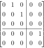 . Then, σ(A) = {0,0,0,0,0}. Note that A
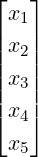 = 0 implies
x2 = 0 = x3 = x5. Thus, e1 and e4 are the only eigenvectors. Note that the diagonal
blocks of A are nilpotent matrices.
= 0 implies
x2 = 0 = x3 = x5. Thus, e1 and e4 are the only eigenvectors. Note that the diagonal
blocks of A are nilpotent matrices.
Exercise 6.1.8.
-
1.
- Let A ∈ Mn(ℝ). Then, prove that
-
(a)
- if α ∈ σ(A) then αk ∈ σ(Ak), for all k ∈ ℕ.
-
(b)
- if A is invertible and α ∈ σ(A) then αk ∈ σ(Ak), for all k ∈ ℤ.
-
2.
- Find eigen-pairs over ℂ, for each of the following matrices:
![[ ]
1 1 + i
1 - i 1](LA1877x.png) ,
, ![[ ]
i 1+ i
- 1+ i i](LA1878x.png) ,
, ![[ ]
cos θ - sin θ
sin θ cos θ](LA1879x.png) and
and ![[ ]
cos θ sin θ
sin θ - cos θ](LA1880x.png) .
.
-
3.
- Let A = [aij] ∈ Mn(ℂ) with ∑
j=1naij = a, for all 1 ≤ i ≤ n. Then, prove that a is an
eigenvalue of A with corresponding eigenvector 1 = [1,1,…,1]T .
-
4.
- Prove that the matrices A and AT have the same set of eigenvalues. Construct a 2 × 2 matrix A
such that the eigenvectors of A and AT are different.
-
5.
- Prove that λ ∈ ℂ is an eigenvalue of A if and only if λ ∈ ℂ is an eigenvalue of A*.

 DRAFT
DRAFT
-
6.
- Let A be an idempotent matrix. Then, prove that its eigenvalues are either 0 or 1 or
both.
-
7.
- Let A be a nilpotent matrix. Then, prove that its eigenvalues are all 0.
-
8.
- Let J = 11T ∈ Mn(ℂ). Then, J is a matrix with each entry 1. Show that
-
(a)
- (n,1) is an eigenpair for J.
-
(b)
- 0 ∈ σ(J) with multiplicity n-1. Find a set of n-1 linearly independent eigenvectors
for 0 ∈ σ(J).
-
9.
- Let B ∈ Mn(ℂ) and C ∈ Mm(ℂ). Now, define the Direct Sum B ⊕C =
![[ ]
B 0
0 C](LA1883x.png) . Then, prove
that
. Then, prove
that
-
(a)
- if (α,x) is an eigen-pair for B then
![( [ ])
α, x
0](LA1884x.png) is an eigen-pair for B ⊕ C.
is an eigen-pair for B ⊕ C.
-
(b)
- if (β,y) is an eigen-pair for C then
![( [ ])
β, 0
y](LA1885x.png) is an eigen-pair for B ⊕ C.
is an eigen-pair for B ⊕ C.
Definition 6.1.9. Let A ∈(ℂn). Then, a vector y ∈ ℂn\{0} satisfying y*A = λy* is called
a left eigenvector of A for λ.
Theorem 6.1.11. [Principle of bi-orthogonality] Let (λ,x) be a (right) eigenpair and (μ,y)
be a left eigenpair of A, where λ≠μ. Then, y is orthogonal to x.
Proof. Verify that μy*x = (y*A)x = y*(λx) = λy*x. Thus, y*x = 0. _
Exercise 6.1.12. Let Ax = λx and x*A = μx*. Then μ = λ.
Definition 6.1.13. [Eigenvalues of a linear Operator] Let T ∈(ℂn). Then, α ∈ is called
an eigenvalue of T if there exists v ∈ ℂn with v≠0 such that T(v) = αv.
is called
an eigenvalue of T if there exists v ∈ ℂn with v≠0 such that T(v) = αv.
Proof. Note that, by definition, T(v) = αv if and only if [Tv] = [αv]. Or equivalently, α ∈ σ(T) if
and only if A[v] = α[v]. Thus, the required result follows. _
= [αv]. Or equivalently, α ∈ σ(T) if
and only if A[v] = α[v]. Thus, the required result follows. _
Remark 6.1.15. [A linear operator on an infinite dimensional space may not have any
eigenvalue] Let V be the space of all real sequences (see Example 3.1.4.8a). Now, define a
linear operator T ∈(V) by
 We now show that T doesn’t have any eigenvalue.
Solution: Let if possible α be an eigenvalue of T with corresponding eigenvector x =
(x1,x2,…). Then, the eigen-condition T(x) = αx implies that
 So, if α≠
0
then x1 = 0
and this in turn implies that x =
0, a contradiction. If α = 0
then
(0
,x1,x2,…) = (0
,0
,…)
and we again get x =
0, a contradiction. Hence, the required result
follows.
Theorem 6.1.16. Let λ1,…,λn, not necessarily distinct, be the A = [aij] ∈ Mn(ℂ). Then,
det(A) = ∏
i=1nλi and tr(A) = ∑
i=1naii = ∑
i=1nλi.

 DRAFT
DRAFT
Proof. Since λ1,…,λn are the eigenvalues of A, by definition,
 | (6.1.2) |
is an identity in x as polynomials. Therefore, by substituting x = 0 in Equation (6.1.2), we get
det(A) = (-1)n(-1)n ∏
i=1nλi = ∏
i=1nλi. Also,
for some a0,a1,…,an-1 ∈ ℂ. Then, an-1, the coefficient of (-1)n-1xn-1, comes from the
term
 So,
an-1 = ∑
i=1naii = tr(A), the trace of A. Also, from Equation (6.1.2) and (6.1.4), we have
So,
an-1 = ∑
i=1naii = tr(A), the trace of A. Also, from Equation (6.1.2) and (6.1.4), we have

 DRAFT
Therefore, comparing the coefficient of (-1)n-1xn-1, we have
DRAFT
Therefore, comparing the coefficient of (-1)n-1xn-1, we have
 Hence, we get the required result. _
Exercise 6.1.17.
-
1.
- Let A be a 3 × 3 orthogonal matrix (AAT = I). If det(A) = 1, then prove that there exists
v ∈ ℝ3 \{0} such that Av = v.
-
2.
- Let A ∈ M2n+1(ℝ) with AT = -A. Then, prove that 0 is an eigenvalue of A.
-
3.
- Let A ∈ Mn(ℂ). Then, A is invertible if and only if 0 is not an eigenvalue of A.
-
4.
- Let A ∈ Mn(ℂ) satisfy ∥Ax∥≤∥x∥ for all x ∈ ℂn. Then, prove that if α ∈ ℂ with |α| > 1
then A - αI is invertible.

 DRAFT
DRAFT
Definition 6.1.18. [Algebraic, Geometric Multiplicity] Let A ∈ Mn(ℂ). Then,
-
1.
- the multiplicity of α ∈ σ(A) is called the algebraic multiplicity of A, denoted
Alg.Mulα(A).
-
2.
- for α ∈ σ(A), dim(Null(A - αI)) is called the geometric multiplicity of A,
Geo.Mulα(A).
We now state the following observations.
Remark 6.1.19. Let A ∈ Mn(ℂ).
-
1.
- Then, for each α ∈ σ(A), using Theorem 2.2.40 dim(Null(A - αI)) ≥ 1. So, we have at
least one eigenvector.
-
2.
- If the algebraic multiplicity of α ∈ σ(A) is r ≥ 2 then the Example 6.1.7.7 implies that
we need not have r linearly independent eigenvectors.
Theorem 6.1.20. Let A and B be two similar matrices. Then,
-
1.
- α ∈ σ(A) if and only if α ∈ σ(B).

 DRAFT
DRAFT
-
2.
- for each α ∈ σ(A), Alg.Mulα(A) = Alg.Mulα(B) and Geo.Mulα(A) =
Geo.Mulα(B).
Proof. Since A and B are similar, there exists an invertible matrix S such that A = SBS-1. So,
α ∈ σ(A) if and only if α ∈ σ(B) as
Note that Equation (6.1.5) also implies that Alg.Mulα(A) = Alg.Mulα(B). We will now show that
Geo.Mulα(A) = Geo.Mulα(B).
So, let Q1 = {v1,…,vk} be a basis of Null(A - αI). Then, B = SAS-1 implies that
Q2 = {Sv1,…,Svk}⊆ Null(B -αI). Since Q1 is linearly independent and S is invertible, we get Q2
is linearly independent. So, Geo.Mulα(A) ≤ Geo.Mulα(B). Now, we can start with eigenvectors of
B and use similar arguments to get Geo.Mulα(B) ≤ Geo.Mulα(A) and hence the required result
follows. _
We will now give a relation between the geometric multiplicity and the algebraic multiplicity.
Theorem 6.1.22. Let A ∈ Mn(ℂ). Then, for α ∈ σ(A), Geo.Mulα(A) ≤ Alg.Mulα(A).
Proof. Let Geo.Mulα(A) = k. Suppose Q1 = {v1,…,vk} is an orthonormal basis of
Null(A - αI). Extend Q1 to get {v1,…,vk,vk+1,…,vn} as an orthonormal basis of ℂn. Put
P = ![[v1,...,vk, vk+1,...,vn]](LA1918x.png) . Then, P* = P-1 and
. Then, P* = P-1 and
Now, if we denote the lower diagonal submatrix as D then
So, Alg.Mulα(A) = Alg.Mulα(P*AP) ≥ k = Geo.Mulα(A). _
Remark 6.1.23. Note that in the proof of Theorem 6.1.22, the remaining eigenvalues of A
are the eigenvalues of D (see Equation (6.1.6)). This technique is called deflation.
Exercise 6.1.24.
-
1.
- Let A =
 . Notice that x
1 =
. Notice that x
1 =  1 is an eigenvector for A. Find an ordered basis
{x1,x2,x3} of ℂ3. Put X =
1 is an eigenvector for A. Find an ordered basis
{x1,x2,x3} of ℂ3. Put X = ![[ ]
x1 x2 x3](LA1925x.png) . Compute X-1AX to get a block-triangular
matrix. Can you now find the remaining eigenvalues of A?
. Compute X-1AX to get a block-triangular
matrix. Can you now find the remaining eigenvalues of A?
-
2.
- Let A ∈ Mm×n(ℝ) and B ∈ Mn×m(ℝ).
-
(a)
- If α ∈ σ(AB) and α≠0 then
-
i.
- α ∈ σ(BA).
-
ii.
- Alg.Mulα(AB) = Alg.Mulα(BA).
-
iii.
- Geo.Mulα(AB) = Geo.Mulα(BA).
-
(b)
- If 0 ∈ σ(AB) and n = m then Alg.Mul0(AB) = Alg.Mul0(BA) as there are n
eigenvalues, counted with multiplicity.
-
(c)
- Give an example to show that Geo.Mul0(AB) need not equal Geo.Mul0(BA) even when
n = m.

 DRAFT
DRAFT
-
3.
- Let A ∈ Mn(ℝ) be an invertible matrix and let x,y ∈ ℝn with x≠0 and yT A-1x≠0. Define
B = xyT A-1. Then, prove that
-
(a)
- λ0 = yT A-1x is an eigenvalue of B of multiplicity 1.
-
(b)
- 0 is an eigenvalue of B of multiplicity n - 1 [Hint: Use Exercise 6.1.24.2a].
-
(c)
- 1 + αλ0 is an eigenvalue of I + αB of multiplicity 1, for any α ∈ ℝ.
-
(d)
- 1 is an eigenvalue of I + αB of multiplicity n - 1, for any α ∈ ℝ.
-
(e)
- det(A + αxyT ) equals (1 + αλ0)det(A), for any α ∈ ℝ. This result is known as the
Shermon-Morrison formula for determinant.
-
4.
- Let A,B ∈ M2(ℝ) such that det(A) = det(B) and tr(A) = tr(B).
-
(a)
- Do A and B have the same set of eigenvalues?
-
(b)
- Give examples to show that the matrices A and B need not be similar.
-
5.
- Let A,B ∈ Mn(ℝ). Also, let (λ1,u) and (λ2,v) are eigen-pairs of A and B, respectively.
-
(a)
- If u = αv for some α ∈ ℝ then (λ1 + λ2,u) is an eigen-pair for A + B.
-
(b)
- Give an example to show that if u and v are linearly independent then λ1 + λ2 need
not be an eigenvalue of A + B.
-
6.
- Let A ∈ Mn(ℝ) be an invertible matrix with eigen-pairs (λ1,u1),…,(λn,un). Then, prove that
 = [u1,…,un] forms a basis of ℝn. If [b] = (c1,…,cn)T then the system Ax = b has the unique
solution
= [u1,…,un] forms a basis of ℝn. If [b] = (c1,…,cn)T then the system Ax = b has the unique
solution
Let A ∈ Mn(ℂ) and let T ∈(ℂn) be defined by T(x) = Ax, for all x ∈ ℂn. In this section, we first
find conditions under which one can obtain a basis of ℂn such that T[,] (see Theorem 4.4.4) is a
diagonal matrix. And, then it is shown that normal matrices satisfy the above conditions. To start
with, we have the following definition.
Definition 6.2.1. [Matrix Diagonalizability] A matrix A is said to be diagonalizable if A
is similar to a diagonal matrix. Or equivalently, P-1AP = D ⇔ AP = PD, for some diagonal
matrix D and invertible matrix P.
Example 6.2.2.
-
1.
- Let A be an n × n diagonalizable matrix. Then, by definition, A is similar to a diagonal
matrix, say D = diag(d1,…,dn). Thus, by Remark 6.1.21, σ(A) = σ(D) = {d1,…,dn}.
-
2.
- Let A =
![[ ]
0 1
0 0](LA1931x.png) . Then, A cannot be diagonalized.
. Then, A cannot be diagonalized.
Solution: Suppose A is diagonalizable. Then, A is similar to D = diag(d1,d2). Thus,
by Theorem 6.1.20, {d1,d2} = σ(D) = σ(A) = {0,0}. Hence, D = 0 and therefore,
A = SDS-1 = 0, a contradiction.
-
3.
- Let A =
 . Then, A cannot be diagonalized.
Solution: Suppose A is diagonalizable. Then, A is similar to D = diag(d1,d2,d3). Thus,
by Theorem 6.1.20, {d1,d2,d3} = σ(D) = σ(A) = {2,2,2}. Hence, D = 2I3 and therefore,
A = SDS-1 = 2I3, a contradiction.

 DRAFT
DRAFT
-
4.
- Let A =
![[ ]
0 1
- 1 0](LA1933x.png) . Then,
. Then, ![( [ ] )
i
i, 1](LA1934x.png) and
and ![( [ ])
- i
- i, 1](LA1935x.png) are two eigen-pairs of A. Define
U =
are two eigen-pairs of A. Define
U = 
![[ ]
i - i
1 1](LA1937x.png) . Then, U*U = I2 = UU* and U*AU =
. Then, U*U = I2 = UU* and U*AU = ![[ ]
- i 0
0 i](LA1938x.png) .
.
Theorem 6.2.3. Let A ∈ Mn(ℝ).
-
1.
- Let S be an invertible matrix such that S-1AS = diag(d1,…,dn). Then, for 1 ≤ i ≤ n,
the i-th column of S is an eigenvector of A corresponding to di.
-
2.
- Then, A is diagonalizable if and only if A has n linearly independent eigenvectors.
Proof. Let S = ![[u1,...,un ]](LA1941x.png) . Then, AS = SD gives
. Then, AS = SD gives
![[Au1,...,Aun ] = A [u1,...,un] = AS = SD = S diag(d1,...,dn) = [d1u1,...,dnun].](LA1942x.png) Or
equivalently, Aui = diui, for 1 ≤ i ≤ n. As S is invertible, {u1,…,un} are linearly independent. Hence,
(di,ui), for 1 ≤ i ≤ n, are eigen-pairs of A. This proves Part 1 and “only if” part of Part
2.
Or
equivalently, Aui = diui, for 1 ≤ i ≤ n. As S is invertible, {u1,…,un} are linearly independent. Hence,
(di,ui), for 1 ≤ i ≤ n, are eigen-pairs of A. This proves Part 1 and “only if” part of Part
2.
Conversely, let {u1,…,un} be n linearly independent eigenvectors of A corresponding
to eigenvalues α1,…,αn. Then, by Corollary 3.3.10, S = ![[u1,...,un ]](LA1943x.png) is non-singular and
is non-singular and
where D = diag(α1,…,αn). Therefore, S-1AS = D and hence A is diagonalizable. _
Definition 6.2.4.
-
1.
- A matrix A ∈ Mn(ℂ) is called defective if for some α ∈ σ(A), Geo.Mulα(A) <
Alg.Mulα(A).
-
2.
- A matrix A ∈ Mn(ℂ) is called non-derogatory if Geo.Mulα(A) = 1, for each α ∈ σ(A).
As a direct consequence of Theorem 6.2.3, we obtain the following result.
Corollary 6.2.5. Let A ∈ Mn(ℂ). Then,
-
1.
- A is non-defective if and only if A is diagonalizable.
-
2.
- A has distinct eigenvalues if and only if A is non-derogatory and non-defective.
Theorem 6.2.6. Let (α1,v1),…,(αk,vk) be k eigen-pairs of A ∈ Mn(ℂ) with αi’s distinct.
Then, {v1,…,vk} is linearly independent.

 DRAFT
DRAFT
Proof. Suppose {v1,…,vk} is linearly dependent. Then, there exists a smallest ℓ ∈{1,…,k - 1} and
β≠0 such that vℓ+1 = β1v1 +  + βℓvℓ. So,
 | (6.2.1) |
and
Now, subtracting Equation (6.2.2) from Equation (6.2.1), we get
 So, vℓ ∈ LS(v1,…,vℓ-1), a contradiction to the choice of ℓ. Thus, the required result
follows. _
So, vℓ ∈ LS(v1,…,vℓ-1), a contradiction to the choice of ℓ. Thus, the required result
follows. _
An immediate corollary of Theorem 6.2.3 and Theorem 6.2.6 is stated next without
proof.

 DRAFT
Corollary 6.2.7. Let A ∈ Mn(ℂ) have n distinct eigenvalues. Then, A is diagonalizable.
DRAFT
Corollary 6.2.7. Let A ∈ Mn(ℂ) have n distinct eigenvalues. Then, A is diagonalizable.
The converse of Theorem 6.2.6 is not true as In has n linearly independent eigenvectors
corresponding to the eigenvalue 1, repeated n times.
Corollary 6.2.8. Let α1,…,αk be k distinct eigenvalues A ∈ Mn(ℂ). Also, for 1 ≤ i ≤ k, let
dim(Null(A - αiIn)) = ni. Then, A has ∑
i=1kni linearly independent eigenvectors.
Proof. For 1 ≤ i ≤ k, let Si = {ui1,…,uini} be a basis of Null(A-αiIn). Then, we need to prove that
⋃
i=1kSi is linearly independent. To do so, denote pj(A) =  ∕
∕ , for
1 ≤ j ≤ k. Then, note that pj(A) is a polynomial in A of degree k - 1 and
, for
1 ≤ j ≤ k. Then, note that pj(A) is a polynomial in A of degree k - 1 and
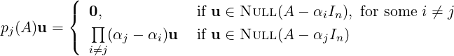 | (6.2.3) |
So, to prove that ⋃
i=1kSi is linearly independent, consider the linear system
 in the variables cij’s. Now, applying the matrix pj(A) and using Equation (6.2.3), we
get
in the variables cij’s. Now, applying the matrix pj(A) and using Equation (6.2.3), we
get

 DRAFT
DRAFT
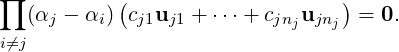 But
∏
i≠j(αj - αi)≠0 as αi’s are distinct. Hence, cj1uj1 +
But
∏
i≠j(αj - αi)≠0 as αi’s are distinct. Hence, cj1uj1 +  + cjnjujnj = 0. As Sj is a basis of
Null(A - αjIn), we get cjt = 0, for 1 ≤ t ≤ nj. Thus, the required result follows. _
+ cjnjujnj = 0. As Sj is a basis of
Null(A - αjIn), we get cjt = 0, for 1 ≤ t ≤ nj. Thus, the required result follows. _
Corollary 6.2.9. Let A ∈ Mn(ℂ) with distinct eigenvalues α1,…,αk. Then, A is diagonalizable
if and only if Geo.Mulαi(A) = Alg.Mulαi(A), for each 1 ≤ i ≤ k.
Proof. Let Alg.Mulαi(A) = mi. Then, ∑
i=1kmi = n. Let Geo.Mulαi(A) = ni, for 1 ≤ i ≤ k. Then,
by Corollary 6.2.8 A has ∑
i=1kni linearly independent eigenvectors. Also, by Theorem 6.1.22,
ni ≤ mi, for 1 ≤ i ≤ mi.
Now, let A be diagonalizable. Then, by Theorem 6.2.3, A has n linearly independent eigenvectors.
So, n = ∑
i=1kni. As ni ≤ mi and ∑
i=1kmi = n, we get ni = mi.
Now, assume that Geo.Mulαi(A) = Alg.Mulαi(A), for 1 ≤ i ≤ k. Then, for each i,1 ≤ i ≤ n, A
has ni = mi linearly independent eigenvectors. Thus, A has ∑
i=1kni = ∑
i=1kmi = n linearly
independent eigenvectors. Hence by Theorem 6.2.3, A is diagonalizable. _
Exercise 6.2.11.

 DRAFT
DRAFT
-
1.
- Let A be diagonalizable. Then, prove that A + αI is diagonalizable for every α ∈ ℂ.
-
2.
- Let A be an strictly upper triangular matrix. Then, prove that A is not diagonalizable.
-
3.
- Let A be an n×n matrix with λ ∈ σ(A) with alg.mulλ(A) = m. If Rank[A-λI]≠n-m
then prove that A is not diagonalizable.
-
4.
- If σ(A) = σ(B) and both A and B are diagonalizable then prove that A is similar to B.
That is, they are two basis representation of the same linear transformation.
-
5.
- Let A and B be two similar matrices such that A is diagonalizable. Prove that B is
diagonalizable.
-
6.
- Let A ∈ Mn(ℝ) and B ∈ Mm(ℝ). Suppose C =
![[ ]
A 0
0 B](LA1968x.png) . Then, prove that C is
diagonalizable if and only if both A and B are diagonalizable.
. Then, prove that C is
diagonalizable if and only if both A and B are diagonalizable.
-
7.
- Is the matrix A =
 diagonalizable?
-
8.
- Let Jn be an n×n matrix with all entries 1. Then, Geo.Mul1(Jn) = Alg.Mul1(Jn) = 1
and Geo.Mul0(Jn) = Alg.Mul0(Jn) = n - 1.
-
9.
- Let A = [aij] ∈ Mn(ℝ), where aij = a, if i = j and b, otherwise. Then, verify that
A = (a - b)In + bJn. Hence, or otherwise determine the eigenvalues and eigenvectors of
Jn. Is A diagonalizable?
-
10.
- Let T : ℝ5-→ℝ5 be a linear operator with Rank(T - I) = 3 and


 DRAFT
DRAFT
-
(a)
- Determine the eigenvalues of T?
-
(b)
- For each distinct eigenvalue α of T, determine Geo.Mulα(T).
-
(c)
- Is T diagonalizable? Justify your answer.
-
11.
- Let A ∈ Mn(ℝ) with A≠0 but A2 = 0. Prove that A cannot be diagonalized.
-
12.
- Are the following matrices diagonalizable?
i)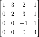 , ii)
, ii)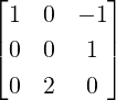 , iii)
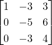 and iv)
![[2 i]
i 0](LA1976x.png) .
.
-
13.
- Let A ∈ Mn(ℂ).
-
(a)
- Then, prove that Rank(A) = 1 if and only if A = xy*, for some non-zero vectors
x,y ∈ ℂn.
-
(b)
- If Rank(A) = 1 then
-
i.
- A has at most one nonzero eigenvalue of algebraic multiplicity 1.
-
ii.
- find this eigenvalue and its geometric multiplicity.
-
iii.
- when is A diagonalizable?
-
14.
- Let A ∈ Mn(ℂ). If Rank(A) = k then there exists xi,yi ∈ ℂn such that A = ∑
i=1kxiyi*. Is the
converse true?
We now prove one of the most important results in diagonalization, called the Schur’s Lemma or the
Schur’s unitary triangularization.

 DRAFT
Lemma 6.2.12 (Schur’s unitary triangularization (SUT)). Let A ∈ Mn(ℂ). Then, there exists
a unitary matrix U such that A is similar to an upper triangular matrix. Further, if A ∈ Mn(ℝ)
and σ(A) have real entries then U is a real orthogonal matrix.
DRAFT
Lemma 6.2.12 (Schur’s unitary triangularization (SUT)). Let A ∈ Mn(ℂ). Then, there exists
a unitary matrix U such that A is similar to an upper triangular matrix. Further, if A ∈ Mn(ℝ)
and σ(A) have real entries then U is a real orthogonal matrix.
Proof. We prove the result by induction on n. The result is clearly true for n = 1. So, let n > 1 and
assume the result to be true for k < n and prove it for n.
Let (λ1,x1) be an eigen-pair of A with ∥x1∥ = 1. Now, extend it to form an orthonormal basis
{x1,x2,…,un} of ℂn and define X = ![[x1,x2,...,un ]](LA1979x.png) . Then, X is a unitary matrix and
. Then, X is a unitary matrix and
where B ∈ Mn-1(ℂ). Now, by induction hypothesis there exists a unitary matrix U ∈ Mn-1(ℂ) such
that U*BU = T is an upper triangular matrix. Define  = X
= X![[ ]
1 0
0 U](LA1982x.png) . Then, using Exercise 5.4.8.10,
the matrix
. Then, using Exercise 5.4.8.10,
the matrix  is unitary and Since T is upper triangular,
 ![[ ]
λ1 *
0 T](LA1985x.png) is upper triangular.
is upper triangular.

 DRAFT
DRAFT
Further, if A ∈ Mn(ℝ) and σ(A) has real entries then x1 ∈ ℝn with Ax1 = λ1x1. Now, one uses
induction once again to get the required result. _
Remark 6.2.13. Let A ∈ Mn(ℂ). Then, by Schur’s Lemma there exists a unitary matrix U such that
U*AU = T = [tij], a triangular matrix. Thus,
 | (6.2.5) |
Furthermore, we can get the αi’s in the diagonal of T in any prescribed order.
Definition 6.2.14. [Unitary Equivalence] Let A,B ∈ Mn(ℂ). Then, A and B are said to be
unitarily equivalent/similar if there exists a unitary matrix U such that A = U*BU.
Remark 6.2.15. We know that if two matrices are unitarily equivalent then they are necessarily
similar as U* = U-1, for every unitary matrix U. But, similarity doesn’t imply unitary equivalence
(see Exercise 6.2.17.6). In numerical calculations, unitary transformations are preferred as compared
to similarity transformations due to the following main reasons:
-
1.
- Exercise 5.4.8.5g implies that ∥Ax∥ = ∥x∥, whenever A is a normal matrix. This need
not be true under a similarity change of basis.

 DRAFT
DRAFT
-
2.
- As U-1 = U*, for a unitary matrix, unitary equivalence is computationally simpler.
-
3.
- Also, computation of “conjugate transpose” doesn’t create round-off error in calculation.
Example 6.2.16. Consider the two matrices A = ![[ ]
3 2
- 1 0](LA1991x.png) and B =
and B = ![[ ]
1 1
0 2](LA1992x.png) . Then, we show
that they are similar but not unitarily similar.
. Then, we show
that they are similar but not unitarily similar.
Solution: Note that σ(A) = σ(B) = {1,2}. As the eigenvalues are distinct, by
Theorem 6.2.7, the matrices A and B are diagonalizable and hence there exists invertible
matrices S and T such that A = SΛS-1, B = TΛT-1, where Λ = ![[ ]
1 0
0 2](LA1993x.png) . Thus,
A = ST-1B(ST-1)-1. That is, A and B are similar. But, ∑
|aij|2≠∑
|bij|2 and hence by
Exercise 5.4.8.11, they cannot be unitarily similar.
. Thus,
A = ST-1B(ST-1)-1. That is, A and B are similar. But, ∑
|aij|2≠∑
|bij|2 and hence by
Exercise 5.4.8.11, they cannot be unitarily similar.
We now use Lemma 6.2.12 to give another proof of Theorem 6.1.16.
Corollary 6.2.18. Let A ∈ Mn(ℂ). If σ(A) = {α1,…,αn} then det(A) = ∏
i=1nαi and
tr(A) = ∑
i=1nαi.
Proof. By Schur’s Lemma there exists a unitary matrix U such that U*AU = T = [tij], a triangular
matrix. By Remark 6.2.13, σ(A) = σ(T). Hence, det(A) = det(T) = ∏
i=1ntii = ∏
i=1nαi and
tr(A) = tr(A(UU*)) = tr(U*(AU)) = tr(T) = ∑
i=1ntii = ∑
i=1nαi. _
We now use Schur’s unitary triangularization Lemma to state the main theorem of this subsection.
Also, recall that A is said to be a normal matrix if AA* = A*A.

 DRAFT
DRAFT
Theorem 6.2.19 (Spectral Theorem for Normal Matrices). Let A ∈ Mn(ℂ). If A is a normal
matrix then there exists a unitary matrix U such that U*AU = diag(α1,…,αn).
Proof. By Schur’s Lemma there exists a unitary matrix U such that U*AU = T = [tij], a triangular
matrix. Since A is a normal
 Thus, we see that T is an upper triangular matrix with T*T = TT*. Thus, by Exercise 1.2.11.4, T is a
diagonal matrix and this completes the proof. _
Thus, we see that T is an upper triangular matrix with T*T = TT*. Thus, by Exercise 1.2.11.4, T is a
diagonal matrix and this completes the proof. _
Exercise 6.2.20. Let A ∈ Mn(ℂ). If A is either a Hermitian, skew-Hermitian or Unitary
matrix then A is a normal matrix.
We re-write Theorem 6.2.19 in another form to indicate that A can be decomposed into linear
combination of orthogonal projectors onto eigen-spaces. Thus, it is independent of the choice of
eigenvectors.
Remark 6.2.21. Let A ∈ Mn(ℂ) be a normal matrix with eigenvalues α1,…,αn.
-
1.
- Then, there exists a unitary matrix U =
![[u1,...,un]](LA2009x.png) such that
such that
-
(a)
- In = u1u1* +
 + unun*.
-
(b)
- the columns of U form a set of orthonormal eigenvectors for A (use Theorem 6.2.3).

 DRAFT
DRAFT
-
(c)
- A = A ⋅ In = A
 = α1u1u1* +
  + αnunun*.
-
2.
- Let α1,…,αk be the distinct eigenvalues of A. Also, let Wi = Null(A-αiIn), for 1 ≤ i ≤ k, be
the corresponding eigen-spaces.
-
(a)
- Then, we can group the ui’s such that they form an orthonormal basis of Wi, for
1 ≤ i ≤ k. Hence, ℂn = W1 ⊕
 ⊕ Wk.
⊕ Wk.
-
(b)
- If Pαi is the orthogonal projector onto Wi, for 1 ≤ i ≤ k then A = α1P1+
 +αkPk.
Thus, A depends only on eigen-spaces and not on the computed eigenvectors.
+αkPk.
Thus, A depends only on eigen-spaces and not on the computed eigenvectors.
We now give the spectral theorem for Hermitian matrices.
Theorem 6.2.22. [Spectral Theorem for Hermitian Matrices] Let A ∈ Mn(ℂ) be a Hermitian
matrix. Then,
-
1.
- the eigenvalues αi, for 1 ≤ i ≤ n, of A are real.
-
2.
- there exists a unitary matrix U, say U =
![[u1,...,un]](LA2017x.png) such that
such that
-
(a)
- In = u1u1* +
 + unun*.
-
(b)
- {u1,…,un} forms a set of orthonormal eigenvectors for A.
-
(c)
- A = α1u1u1* +
 + αnunun*, or equivalently, U*AU = D, where D =
diag(α1,…,αn).
+ αnunun*, or equivalently, U*AU = D, where D =
diag(α1,…,αn).
Proof. The second part is immediate from Theorem 6.2.19 as Hermitian matrices are also normal
matrices. For Part 1, let (α,x) be an eigen-pair. Then, Ax = αx. As A is Hermitian A* = A. Thus,
x*A = x*A* = (Ax)* = (αx)* = αx*. Hence, using x*A = αx*, we get

 DRAFT
DRAFT
 As x
is an eigenvector, x≠0. Hence, ∥x∥2 = x*x≠0. Thus α = α, i.e., α ∈ ℝ. _
As x
is an eigenvector, x≠0. Hence, ∥x∥2 = x*x≠0. Thus α = α, i.e., α ∈ ℝ. _
As an immediate corollary of Theorem 6.2.22 and the second part of Lemma 6.2.12, we give the
following result without proof.
Corollary 6.2.23. Let A ∈ Mn(ℝ) be symmetric. Then, A = U diag(α1,…,αn) U*, where
-
1.
- the αi’s are all real,
-
2.
- the columns of U can be chosen to have real entries,
-
3.
- the eigenvectors that correspond to the columns of U form an orthonormal basis of ℝn.
Exercise 6.2.24.
-
1.
- Let A be a skew-symmetric matrix. Then, the eigenvalues of A are either zero or purely
imaginary and A is unitarily diagonalizable.
-
2.
- Let A be a skew-Hermitian matrix. Then, A is unitarily diagonalizable.
-
3.
- Characterize all normal matrices in M2(ℝ).
-
4.
- Let σ(A) = {λ1,…,λn}. Then, prove that the following statements are equivalent.

 DRAFT
DRAFT
-
(a)
- A is normal.
-
(b)
- A is unitarily diagonalizable.
-
(c)
- ∑
i,j|aij|2 = ∑
i|λi|2.
-
(d)
- A has n orthonormal eigenvectors.
-
5.
- Let A be a normal matrix with (λ,x) as an eigen-pair. Then,
-
(a)
- (A*)kx for k ∈ ℤ+ is also an eigenvector corresponding to λ.
-
(b)
- (λ,x) is an eigen-pair for A*. [Hint: Verify ∥A*x -λx∥2 = ∥Ax - λx∥2.]
-
6.
- Let A be an n × n unitary matrix. Then,
-
(a)
- |λ| = 1 for any eigenvalue λ of A.
-
(b)
- the eigenvectors x,y corresponding to distinct eigenvalues are orthogonal.
-
7.
- Let A be a 2 × 2 orthogonal matrix. Then, prove the following:
-
(a)
- if det(A) = 1 then A =
![[ ]
cosθ - sin θ
sin θ cosθ](LA2025x.png) , for some θ,0 ≤ θ < 2π. That is, A
counterclockwise rotates every point in ℝ2 by an angle θ.
, for some θ,0 ≤ θ < 2π. That is, A
counterclockwise rotates every point in ℝ2 by an angle θ.
-
(b)
- if detA = -1 then A =
![[ ]
cosθ sin θ
sin θ - cosθ](LA2026x.png) , for some θ,0 ≤ θ < 2π. That is, A
reflects every point in ℝ2 about a line passing through origin. Determine this line.
Or equivalently, there exists a non-singular matrix P such that P-1AP =
, for some θ,0 ≤ θ < 2π. That is, A
reflects every point in ℝ2 about a line passing through origin. Determine this line.
Or equivalently, there exists a non-singular matrix P such that P-1AP = ![[ ]
1 0
0 - 1](LA2027x.png) .
.
-
8.
- Let A be a 3 × 3 orthogonal matrix. Then, prove the following:
-
(a)
- if det(A) = 1 then A is a rotation about a fixed axis, in the sense that A has an
eigen-pair (1,x) such that the restriction of A to the plane x⊥ is a two dimensional
rotation in x⊥.

 DRAFT
DRAFT
-
(b)
- if detA = -1 then A corresponds to a reflection through a plane P, followed by a
rotation about the line through origin that is orthogonal to P.
-
9.
- Let A be a normal matrix. Then, prove that Rank(A) equals the number of nonzero eigenvalues
of A.
-
10.
- [Equivalent characterizations of Hermitian matrices] Let A ∈ Mn(ℂ). Then, the following
statements are equivalent.
-
(a)
- The matrix A is Hermitian.
-
(b)
- The number x*Ax is real for each x ∈ ℂn.
-
(c)
- The matrix A is normal and has real eigenvalues.
-
(d)
- The matrix S*AS is Hermitian for each S ∈ Mn(ℂ).
Let A ∈ Mn(ℂ). Then, in Theorem 6.1.16, we saw that
 | (6.2.6) |
for certain ai ∈ ℂ, 0 ≤ i ≤ n - 1. Also, if α is an eigenvalue of A then PA(α) = 0. So,
xn - an-1xn-1 + an-2xn-2 +  + (-1)n-1a1x + (-1)na0 = 0 is satisfied by n complex numbers. It
turns out that the expression
+ (-1)n-1a1x + (-1)na0 = 0 is satisfied by n complex numbers. It
turns out that the expression

 DRAFT
DRAFT
 holds
true as a matrix identity. This is a celebrated theorem called the Cayley Hamilton Theorem. We
give a proof using Schur’s unitary triangularization. To do so, we look at multiplication of certain
upper triangular matrices.
holds
true as a matrix identity. This is a celebrated theorem called the Cayley Hamilton Theorem. We
give a proof using Schur’s unitary triangularization. To do so, we look at multiplication of certain
upper triangular matrices.
Lemma 6.2.25. Let A1,…,An ∈ Mn(ℂ) be upper triangular matrices such that the (i,i)-th
entry of Ai equals 0, for 1 ≤ i ≤ n. Then, A1A2 An = 0.
Proof. We use induction to prove that the first k columns of A1A2 Ak is 0, for 1 ≤ k ≤ n. The result
is clearly true for k = 1 as the first column of A1 is 0. For clarity, we show that the first two columns
of A1A2 is 0. Let B = A1A2. Then, by matrix multiplication
Ak is 0, for 1 ≤ k ≤ n. The result
is clearly true for k = 1 as the first column of A1 is 0. For clarity, we show that the first two columns
of A1A2 is 0. Let B = A1A2. Then, by matrix multiplication
![B [:,i] = A1[:,1](A2)1i + A1[:,2](A2)2i + ⋅⋅⋅+ A1 [:,n](A2 )ni = 0 + ⋅⋅⋅+ 0 = 0](LA2037x.png) as
A1[:,1] = 0 and (A2)ji = 0, for i = 1,2 and j ≥ 2. So, assume that the first n - 1 columns of
C = A1
as
A1[:,1] = 0 and (A2)ji = 0, for i = 1,2 and j ≥ 2. So, assume that the first n - 1 columns of
C = A1 An-1 is 0 and let B = CAn. Then, for 1 ≤ i ≤ n, we see that
![B [:,i] = C[:,1](A ) + C [:,2](A ) + ⋅⋅⋅+ C [:,n](A ) = 0 + ⋅⋅⋅+ 0 = 0
n 1i n 2i n ni](LA2039x.png) as
C[:,j] = 0, for 1 ≤ j ≤ n - 1 and (An)ni = 0, for i = n - 1,n. Thus, by induction hypothesis the
required result follows. _
as
C[:,j] = 0, for 1 ≤ j ≤ n - 1 and (An)ni = 0, for i = n - 1,n. Thus, by induction hypothesis the
required result follows. _

 DRAFT
DRAFT
Exercise 6.2.26. Let A,B ∈ Mn(ℂ) be upper triangular matrices with the top leading principal
submatrix of A of size k being 0. If B[k + 1,k + 1] = 0 then prove that the leading principal
submatrix of size k + 1 of AB is 0.
We now prove the Cayley Hamilton Theorem using Schur’s unitary triangularization.
Theorem 6.2.27 (Cayley Hamilton Theorem). Let A ∈ Mn(ℂ). Then, A satisfies its
characteristic equation. That is, if PA(x) = det(A-xIn) = a0-xa1+ +(-1)n-1an-1xn-1+
(-1)nxn then
+(-1)n-1an-1xn-1+
(-1)nxn then
 holds true as a matrix identity.
Proof. Let σ(A) = {α1,…,αn} then PA(x) = ∏
i=1n(x-αi). And, by Schur’s unitary triangularization
there exists a unitary matrix U such that U*AU = T, an upper triangular matrix with tii = αi, for
1 ≤ i ≤ n. Now, observe that if Ai = T - αiI then the Ai’s satisfy the conditions of Lemma 6.2.25.
Hence,
 Therefore,

 DRAFT
DRAFT
![∏n ∏n
PA(A ) = (A - αiI) = (U TU * - αiU IU*) = U [(T - α1I) ⋅⋅⋅(T - αnI )]U * = U 0U * = 0.
i=1 i=1](LA2047x.png) Thus, the required result follows. _
Thus, the required result follows. _
We now give some examples and then implications of the Cayley Hamilton Theorem.
Remark 6.2.28.
-
1.
- Let A =
![[ ]
1 2
1 - 3](LA2048x.png) . Then, PA(x) = x2 + 2x - 5. Hence, verify that
. Then, PA(x) = x2 + 2x - 5. Hence, verify that
![[ 3 - 4] [1 2 ] [1 0]
A2 + 2A - 5I2 = + 2 - 5 = 0.
- 2 11 1 - 3 0 1](LA2049x.png) Further, verify that A-1 =
Further, verify that A-1 = 
 =
= 
![[ ]
3 2
1 - 1](LA2053x.png) . Furthermore, A2 = -2A + 5I
implies that
. Furthermore, A2 = -2A + 5I
implies that

 DRAFT
" class="math-display" > We can keep using the above technique to get Am as a linear combination of A and I, for
all m ≥ 1.
DRAFT
" class="math-display" > We can keep using the above technique to get Am as a linear combination of A and I, for
all m ≥ 1.
-
2.
- Let A =
![[ ]
3 1
2 0](LA2057x.png) . Then, PA(t) = t(t- 3) - 2 = t2 - 3t- 2. So, using PA(A) = 0, we have
A-1 =
. Then, PA(t) = t(t- 3) - 2 = t2 - 3t- 2. So, using PA(A) = 0, we have
A-1 =  . Further, A2 = 3A + 2I implies that A3 = 3A2 + 2A = 3(3A + 2I) + 2A =
11A + 6I. So, as above, Am is a combination of A and I, for all m ≥ 1.
. Further, A2 = 3A + 2I implies that A3 = 3A2 + 2A = 3(3A + 2I) + 2A =
11A + 6I. So, as above, Am is a combination of A and I, for all m ≥ 1.
-
3.
- Let A =
![[ ]
0 1
0 0](LA2059x.png) . Then, PA(x) = x2. So, even though A≠0, A2 = 0.
. Then, PA(x) = x2. So, even though A≠0, A2 = 0.
-
4.
- For A =
 , P
A(x) = x3. Thus, by the Cayley Hamilton Theorem A3 = 0. But,
it turns out that A2 = 0.
, P
A(x) = x3. Thus, by the Cayley Hamilton Theorem A3 = 0. But,
it turns out that A2 = 0.
-
5.
- For A =
 , note that P
A(t) = (t - 1)3. So PA(A) = 0. But, observe that if
q(t) = (t - 1)2 then q(A) is also 0.
, note that P
A(t) = (t - 1)3. So PA(A) = 0. But, observe that if
q(t) = (t - 1)2 then q(A) is also 0.
-
6.
- Let A ∈ Mn(ℂ) with PA(x) = a0 - xa1 +
 + (-1)n-1an-1xn-1 + (-1)nxn.
-
(a)
- Then, for any ℓ ∈ ℕ, the division algorithm gives α0,α1,…,αn-1 ∈ ℂ and a polynomial
f(x) with coefficients from ℂ such that
 Hence, by the Cayley Hamilton Theorem, Aℓ = α0I + α1A +
  + αn-1An-1.
-
i.
- Thus, to compute any power of A, one needs to apply the division algorithm to
get αi’s and know Ai, for 1 ≤ i ≤ n - 1. This is quite helpful in numerical
computation as computing powers takes much more time than division.

 DRAFT
DRAFT
-
ii.
- Note that LS
 is a subspace of Mn(ℂ). Also, dim
 = n2.
But, the above argument implies that dim
= n2.
But, the above argument implies that dim ≤ n.
≤ n.
-
iii.
- In the language of graph theory, it says the following: “Let G be a graph on n
vertices and A its adjacency matrix. Suppose there is no path of length n - 1 or
less from a vertex v to a vertex u in G. Then, G doesn’t have a path from v to u
of any length. That is, the graph G is disconnected and v and u are in different
components of G.”
-
(b)
- Suppose A is non-singular. Then, by definition a0 = det(A)≠0. Hence,
![- 1 1 [ n-2 n-2 n-1 n-1]
A = a--a1I - a2A + ⋅⋅⋅+ (- 1) an- 1A + (- 1) A .
0](LA2070x.png) This matrix identity can be used to calculate the inverse.
This matrix identity can be used to calculate the inverse.
-
(c)
- The above also implies that if A is invertible then A-1 ∈ LS
 . That is, A-1 is
a linear combination of the vectors I,A,…,An-1.
. That is, A-1 is
a linear combination of the vectors I,A,…,An-1.
The next section deals with quadratic forms which helps us in better understanding of conic
sections in analytic geometry.
Definition 6.3.1. [Positive, Semi-positive and Negative definite matrices] Let A ∈ Mn(ℂ). Then,
A is said to be

 DRAFT
DRAFT
-
1.
- positive semi-definite (psd) if x*Ax ∈ ℝ and x*Ax ≥ 0, for all x ∈ ℂn.
-
2.
- positive definite (pd) if x*Ax ∈ ℝ and x*Ax > 0, for all x ∈ ℂn \{0}.
-
3.
- negative semi-definite (nsd) if x*Ax ∈ ℝ and x*Ax ≤ 0, for all x ∈ ℂn.
-
4.
- negative definite (nd) if x*Ax ∈ ℝ and x*Ax < 0, for all x ∈ ℂn \{0}.
-
5.
- indefinite if x*Ax ∈ ℝ and there exist x,y ∈ ℂn such that x*Ax < 0 < y*Ay.
Lemma 6.3.2. Let A ∈ Mn(ℂ). Then A is Hermitian if and only if at least one of the following
statements hold:
-
1.
- S*AS is Hermitian for all S ∈ Mn.
-
2.
- A is normal and has real eigenvalues.
-
3.
- x*Ax ∈ ℝ for all x ∈ ℂn.
Proof. Let S ∈ Mn, (S*AS)* = S*A*S = S*AS. Thus S*AS is Hermitian.
Suppose A = A*. Then, A is clearly normal as AA* = A2 = A*A. Further, if (λ,x) is an eigenpair
then λx*x = x*Ax ∈ ℝ implies λ ∈ ℝ.
For the last part, note that x*Ax ∈ ℂ. Thus x*Ax = (x*Ax)* = x*A*x = x*Ax, we get
Im(x*Ax) = 0. Thus, x*Ax ∈ ℝ.
If S*AS is Hermitian for all S ∈ Mn then taking S = In gives A is Hermitian.
If A is normal then A = U* diag(λ1,…,λn)U for some unitary matrix U. Since λi ∈ ℝ,
A* = (U* diag(λ1,…,λn)U)* = U* diag(λ1,…,λn)U = U* diag(λ1,…,λn)U = A. So, A is
Hermitian.
If x*Ax ∈ ℝ for all x ∈ ℂn then aii = ei*Aei ∈ ℝ. Also, aii + ajj + aij + aji = (ei + ej)*A(ei + ej) ∈ ℝ.
So, Im(aij) = -Im(aji). Similarly, aii + ajj + iaij - iaji = (ei + iej)*A(ei + iej) ∈ ℝ implies that
Re(aij) = Re(aji). Thus, A = A*. _

 DRAFT
Remark 6.3.3. Let A ∈ Mn(ℝ). Then the condition x*Ax ∈ ℝ in Definition 6.3.9 is always
true and hence doesn’t put any restriction on the matrix A. So, in Definition 6.3.9, we assume
that AT = A, i.e., A is a symmetric matrix.
DRAFT
Remark 6.3.3. Let A ∈ Mn(ℝ). Then the condition x*Ax ∈ ℝ in Definition 6.3.9 is always
true and hence doesn’t put any restriction on the matrix A. So, in Definition 6.3.9, we assume
that AT = A, i.e., A is a symmetric matrix.
Theorem 6.3.5. Let A ∈ Mn(ℂ). Then, the following statements are equivalent.
-
1.
- A is positive semi-definite.
-
2.
- A* = A and each eigenvalue of A is non-negative.
-
3.
- A = B*B for some B ∈ Mn(ℂ).
Proof. 1 ⇒2: Let A be positive semi-definite. Then, by Lemma 6.3.2 A is Hermitian. If (α,v) is an
eigen-pair of A then α∥v∥2 = v*Av ≥ 0. So, α ≥ 0.

 DRAFT
DRAFT
2 ⇒3: Let σ(A) = {α1,…,αn}. Then, by spectral theorem, there exists a unitary matrix U such
that U*AU = D with D = diag(α1,…,αn). As αi ≥ 0, for 1 ≤ i ≤ n, define D = diag(
 ,…,
,…, ).
Then, A = UD
).
Then, A = UD [D
[D U*] = B*B.
3 ⇒1: Let A = B*B. Then, for x ∈ ℂn, x*Ax = x*B*Bx = ∥Bx∥2 ≥ 0. Thus, the required
result follows. _
A similar argument gives the next result and hence the proof is omitted.
Theorem 6.3.6. Let A ∈ Mn(ℂ). Then, the following statements are equivalent.
-
1.
- A is positive definite.
-
2.
- A* = A and each eigenvalue of A is positive.
-
3.
- A = B*B for a non-singular matrix B ∈ Mn(ℂ).
Remark 6.3.7. Let A ∈ Mn(ℂ) be a Hermitian matrix with eigenvalues λ1 ≥ λ2 ≥ ≥ λn. Then,
there exists a unitary matrix U = [u1,u2,…,un] and a diagonal matrix D = diag(λ1,λ2,…,λn) such
that A = UDU*. Now, for 1 ≤ i ≤ n, define αi = max{λi,0} and βi = min{λi,0}. Then
≥ λn. Then,
there exists a unitary matrix U = [u1,u2,…,un] and a diagonal matrix D = diag(λ1,λ2,…,λn) such
that A = UDU*. Now, for 1 ≤ i ≤ n, define αi = max{λi,0} and βi = min{λi,0}. Then
-
1.
- for D1 = diag(α1,α2,…,αn), the matrix A1 = UD1U* is positive semi-definite.
-
2.
- for D2 = diag(β1,β2,…,βn), the matrix A2 = UD2U* is positive semi-definite.
-
3.
- A = A1 - A2. The matrix A1 is generally called the positive semi-definite part of A.
Definition 6.3.8. [Multilinear Function] Let V be a vector space over F. Then,

 DRAFT
DRAFT
-
1.
- for a fixed m ∈ ℕ, a function f : Vm → F is called an m-multilinear function if f is linear in
each component. That is, for α ∈ F, u ∈ V and vi ∈ V, for 1 ≤ i ≤ m.
-
2.
- An m-multilinear form is also called an m-form.
-
3.
- A 2-form is called a bilinear form.
Definition 6.3.9. [Sesquilinear, Hermitian and Quadratic Forms] Let A = [aij] ∈ Mn(ℂ)
be a Hermitian matrix and let x,y ∈ ℂn. Then, a sesquilinear form in x,y ∈ ℂn is defined as
H(x,y) = y*Ax. In particular, H(x,x), denoted H(x), is called a Hermitian form. In case
A ∈ Mn(ℝ), H(x) is called a quadratic form.
Remark 6.3.10. Observe that
-
1.
- if A = In then the bilinear/sesquilinear form reduces to the standard inner product.
-
2.
- H(x,y) is ‘linear’ in the first component and ‘conjugate linear’ in the second component.

 DRAFT
DRAFT
-
3.
- the quadratic form H(x) is a real number. Hence, for α ∈ ℝ, the equation H(x) = α,
represents a conic in ℝn.
Example 6.3.11.
-
1.
- Let vi ∈ ℂn, for 1 ≤ i ≤ n. Then, f
 = det
= det![([v1,...,vn])](LA2117x.png) is an n-form on ℂn.
is an n-form on ℂn.
-
2.
- Let A ∈ Mn(ℝ). Then, f(x,y) = yT Ax, for x,y ∈ ℝn, is a bilinear form on ℝn.
-
3.
- Let A =
![[ ]
1 2 - i
2 + i 2](LA2118x.png) . Then, A* = A and for x =
. Then, A* = A and for x = ![[ ]
x
y](LA2119x.png) , verify that
, verify that
 where ‘Re’ denotes the real part of a complex number, is a sesquilinear form.
The main idea of this section is to express H(x) as sum or difference of squares. Since H(x) is a
quadratic in x, replacing x by cx, for c ∈ ℂ, just gives a multiplication factor by |c|2. Hence, one needs
to study only the normalized vectors. Let us consider Example 6.1.1 again. There we see that
Note that both the expressions in Equation (6.3.1) is the difference of two non-negative terms.
Whereas, both the expressions in Equation (6.3.2) consists of sum of two non-negative terms. Is this
just a coincidence?
In general, let A ∈ Mn(ℂ) be a Hermitian matrix. Then, by Theorem 6.2.22, σ(A) = {α1,…,αn}⊆ ℝ
and there exists a unitary matrix U such that U*AU = D = diag(α1,…,αn). Let x = Uz. Then,
∥x∥ = 1 and U is unitary implies that ∥z∥ = 1. If z = (z1,…,zn)* then
 | (6.3.3) |
where α1,…,αp > 0, αp+1,…,αr < 0 and αr+1,…,αn = 0. Thus, we see that the possible values of
H(x) seem to depend only on the eigenvalues of A. Since U is an invertible matrix, the
components zi’s of z = U-1x = U*x are commonly known as the linearly independent
linear forms. Note that each zi is a linear expression in the components of x. Also, note
that in Equation (6.3.3), p corresponds to the number of positive eigenvalues and r - p to
the number of negative eigenvalues. For a better understanding, we define the following
numbers.
Definition 6.3.12. [Inertia and Signature of a Matrix] Let A ∈ Mn(ℂ) be a Hermitian
matrix. The inertia of A, denoted i(A), is the triplet (i+(A),i-(A),i0(A)), where i+(A) is the
number of positive eigenvalues of A, i-(A) is the number of negative eigenvalues of A and i0(A)
is the nullity of A. The difference i+(A) - i-(A) is called the signature of A.

 DRAFT
DRAFT
Exercise 6.3.13. Let A ∈ Mn(ℂ) be a Hermitian matrix. If the signature and the rank of A
is known then prove that one can find out the inertia of A.
As a next result, we show that in any expression of H(x) as a sum or difference of n absolute
squares of linearly independent linear forms, the number p (respectively, r - p) gives the number of
positive (respectively, negative) eigenvalues of A. This is popularly known as the ‘Sylvester’s law of
inertia’.
Lemma 6.3.14. [Sylvester’s Law of Inertia] Let A ∈ Mn(ℂ) be a Hermitian matrix and let
x ∈ ℂn. Then, every Hermitian form H(x) = x*Ax, in n variables can be written as
 where y1,…,yr are linearly independent linear forms in the components of x and the integers
p and r satisfying
where y1,…,yr are linearly independent linear forms in the components of x and the integers
p and r satisfying 0
≤ p ≤ r ≤ n, depend only on A.
Proof. Equation (6.3.3) implies that H(x) has the required form. We only need to show that p and r
are uniquely determined by A. Hence, let us assume on the contrary that there exist p,q,r,s ∈ ℕ with
p > q such that
where
y =
![[ ]
Y1
Y2](LA2129x.png)
=
Mx,
z =
![[ ]
Z1
Z2](LA2130x.png)
=
Nx with
Y 1 =
and
Z1 =
for some invertible
matrices
M and
N. Now the invertibility of
M and
N implies
z =
By, for some invertible matrix
B.
Decompose
B =
![[ ]
B1 B2
B3 B4](LA2133x.png) ,
, where
B1 is a
q ×p matrix. Then
![[ ]
Z1
Z2](LA2134x.png)
=
![[ ]
B1 B2
B3 B4](LA2135x.png)
![[ ]
Y1
Y2](LA2136x.png)
. As
p > q, the
homogeneous linear system
B1Y 1 =
0 has a nontrivial solution, say

=
and consider

=
![[^ ]
Y1
0](LA2140x.png)
. Then for this choice of

,
Z1 =
0 and thus, using Equations (
6.3.4) and (
6.3.5), we
have

Now, this can hold only if  = 0, a contradiction to
  being a non-trivial solution.
Hence p = q. Similarly, the case r > s can be resolved. This completes the proof of the
lemma. __
being a non-trivial solution.
Hence p = q. Similarly, the case r > s can be resolved. This completes the proof of the
lemma. __
Remark 6.3.15. Since A is Hermitian, Rank(A) equals the number of nonzero eigenvalues.
Hence, Rank(A) = r. The number r is called the rank and the number r - 2p is called the
inertial degree of the Hermitian form H(x).

 DRAFT
DRAFT
We now look at another form of the Sylvester’s law of inertia. We start with the following
definition.
Definition 6.3.16. [Star Congruence] Let A,B ∈ Mn(ℂ). Then, A is said to be *-congruent
(read star-congruent) to B if there exists an invertible matrix S such that A = S*BS.
Theorem 6.3.17. [Second Version: Sylvester’s Law of Inertia] Let A,B ∈ Mn(ℂ) be
Hermitian. Then, A is *-congruent to B if and only if i(A) = i(B).
Proof. By spectral theorem U*AU = ΛA and V *BV = ΛB, for some unitary matrices U,V and
diagonal matrices ΛA,ΛB of the form diag(+, ,+,-,
,+,-, ,-,0,
,-,0, ,0). Thus, there exist invertible
matrices S,T such that S*AS = DA and T*BT = DB, where DA,DB are diagonal matrices of the
form diag(1,
,0). Thus, there exist invertible
matrices S,T such that S*AS = DA and T*BT = DB, where DA,DB are diagonal matrices of the
form diag(1, ,1,-1,
 ,-1,0,
 ,0).
,0).
If i(A) = i(B), then it follows that DA = DB, i.e., S*AS = T*BT and hence A = (TS-1)*B(TS-1).
Conversely, suppose that A = P*BP, for some invertible matrix P, and i(B) = (k,l,m). As
T*BT = DB, we have, A = P*(T*)-1DBT-1P = (T-1P)*DB(T-1P). Now, let X = (T-1P)-1. Then,
A = (X-1)*DBX-1 and we have the following observations.
-
1.
- As rank and nullity do not change under similarity transformation, i0(A) = i0(DB) = m
as i(B) = (k,l,m).
-
2.
- Using i(B) = (k,l,m), we also have
![* * - 1* -1 *
X [:,k + 1]AX [:,k + 1] = X [:,k + 1] ((X )DB (X ))X [:,k + 1] = ek+1DBek+1 = - 1.
<img
src=](LA2155x.png)
 DRAFT
" class="math-display" > Similarly, X[:,k + 2]*AX[:,k + 2] =
DRAFT
" class="math-display" > Similarly, X[:,k + 2]*AX[:,k + 2] =  = X[:,k + l]*AX[:,k + l] = -1. As the vectors
X[:,k + 1],…,X[:,k + l] are linearly independent, using 9.7.10, we see that A has at least
l negative eigenvalues.
= X[:,k + l]*AX[:,k + l] = -1. As the vectors
X[:,k + 1],…,X[:,k + l] are linearly independent, using 9.7.10, we see that A has at least
l negative eigenvalues.
-
3.
- Similarly, X[:,1]*AX[:,1] =
 = X[:,k]*AX[:,k] = 1. As X[:,1],…,X[:,k] are linearly
independent, using 9.7.10 again, we see that A has at least k positive eigenvalues.
= X[:,k]*AX[:,k] = 1. As X[:,1],…,X[:,k] are linearly
independent, using 9.7.10 again, we see that A has at least k positive eigenvalues.
Thus, it now follows that i(A) = (k,l,m). _
We now obtain conditions on the eigenvalues of A, corresponding to the associated quadratic form, to
characterize conic sections in ℝ2, with respect to the standard inner product.
Definition 6.3.18. [Associated Quadratic Form] Let f(x,y) = ax2+2hxy+by2+2fx+2gy+c
be a general quadratic in x and y, with coefficients from ℝ. Then,
![[ ] [ ]
T [ ] a h x 2 2
H (x) = x Ax = x, y h b y = ax + 2hxy + by](LA2160x.png)
is called the
associated quadratic form of the conic
f(
x,y) = 0.
Proposition 6.3.19. Consider the general quadratic f(x,y), for a,b,c,g,f,h ∈ ℝ. Then, f(x,y) = 0
represents
-
1.
- an ellipse or a circle if ab - h2 > 0,

 DRAFT
DRAFT
-
2.
- a parabola or a pair of parallel lines if ab - h2 = 0,
-
3.
- a hyperbola or a pair of intersecting lines if ab - h2 < 0.
Proof. As A is symmetric, by Corollary 6.2.23, A = U diag(α1,α2)UT , where U = ![[u1,u2]](LA2163x.png) is an
orthogonal matrix, with (α1,u1) and (α2,u2) as eigen-pairs of A. Let
is an
orthogonal matrix, with (α1,u1) and (α2,u2) as eigen-pairs of A. Let ![[u,v]](LA2164x.png) = xT U. As u1 and u2 are
orthogonal, u and v represent orthogonal lines passing through origin in the (x,y)-plane. In most
cases, these lines form the principal axes of the conic.
= xT U. As u1 and u2 are
orthogonal, u and v represent orthogonal lines passing through origin in the (x,y)-plane. In most
cases, these lines form the principal axes of the conic.
We also have xT Ax = α1u2 + α2v2 and hence f(x,y) = 0 reduces to
 | (6.3.6) |
for some g1,f1 ∈ ℝ. Now, we consider different cases depending of the values of α1,α2:
-
1.
- If α1 = 0 = α2 then A = 0 and Equation (6.3.6) gives the straight line 2gx+2fy +c = 0.
-
2.
- if α1 = 0 and α2≠0 then ab-h2 = det(A) = α1α2 = 0. So, after dividing by α2, Equation (6.3.6)
reduces to (v + d1)2 = d2u + d3, for some d1,d2,d3 ∈ ℝ. Hence, let us look at the possible
subcases:
-
(a)
- Let d2 = d3 = 0. Then, v + d1 = 0 is a pair of coincident lines.
-
(b)
- Let d2 = 0,d3≠0.
-
i.
- If d3 > 0, then we get a pair of parallel lines given by v = -d1 ±
 .
.
-
ii.
- If d3 < 0, the solution set of the corresponding conic is an empty set.
-
(c)
- If d2≠0. Then, the given equation is of the form Y 2 = 4aX for some translates X = x + α
and Y = y + β and thus represents a parabola.

 DRAFT
DRAFT
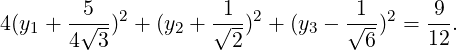
Let H(x) = x2 + 4y2 + 4xy be the associated quadratic form for a class of curves. Then,
A = ![[ ]
1 2
2 4](LA2167x.png) , α1 = 0,α2 = 5 and v = x + 2y. Now, let d1 = -3 and vary d2 and d3 to get
different curves (see Figure 6.2 drawn using the package “MATHEMATICA”).
, α1 = 0,α2 = 5 and v = x + 2y. Now, let d1 = -3 and vary d2 and d3 to get
different curves (see Figure 6.2 drawn using the package “MATHEMATICA”).
-
3.
- α1 > 0 and α2 < 0. Then, ab - h2 = det(A) = λ1λ2 < 0. If α2 = -β2, for β2 > 0, then
Equation (6.3.6) reduces to
 | (6.3.7) |
whose understanding requires the following subcases:

 DRAFT
DRAFT
-
(a)
- If d3 = 0 then Equation (6.3.7) equals
 or equivalently, a pair of intersecting straight lines u + d1 = 0 and v + d2 = 0 in the
(u,v)-plane.
or equivalently, a pair of intersecting straight lines u + d1 = 0 and v + d2 = 0 in the
(u,v)-plane.
-
(b)
- Without loss of generality, let d3 > 0. Then, Equation (6.3.7) equals
 or equivalently, a hyperbola with orthogonal principal axes u+d1 = 0 and v+d2 = 0.
Let H(x) = 10x2 - 5y2 + 20xy be the associated quadratic form for a class of curves. Then,
A = ![[ ]
10 10
10 - 5](LA2178x.png) , α1 = 15,α2 = -10 and
, α1 = 15,α2 = -10 and  u = 2x + y,
 v = x - 2y. Now, let
d1 =
v = x - 2y. Now, let
d1 =  ,d2 = -
 to get 3(2x + y + 1)2 - 2(x - 2y - 1)2 = d3. Now vary d3 to get
different curves (see Figure 6.3 drawn using the package ”MATHEMATICA”).
to get 3(2x + y + 1)2 - 2(x - 2y - 1)2 = d3. Now vary d3 to get
different curves (see Figure 6.3 drawn using the package ”MATHEMATICA”).
-
4.
- α1,α2 > 0. Then, ab - h2 = det(A) = α1α2 > 0 and Equation (6.3.6) reduces to
 | (6.3.8) |
We consider the following three subcases to understand this.
-
(a)
- If d3 = 0 then we get a pair of orthogonal lines u + d1 = 0 and v + d2 = 0.
-
(b)
- If d3 < 0 then the solution set of Equation (6.3.8) is an empty set.
-
(c)
- If d3 > 0 then Equation (6.3.8) reduces to
 +
+ = 1, an ellipse
or circle with u + d1 = 0 and v + d2 = 0 as the orthogonal principal axes.
= 1, an ellipse
or circle with u + d1 = 0 and v + d2 = 0 as the orthogonal principal axes.
Let H(x) = 6x2 + 9y2 + 4xy be the associated quadratic form for a class of curves. Then,
A = ![[ ]
6 2
2 9](LA2193x.png) , α1 = 10,α2 = 5 and
, α1 = 10,α2 = 5 and  u = x + 2y,
 v = 2x-y. Now, let d1 =
  ,d2 = -
 to
get 2(x + 2y + 1)2 + (2x - y - 1)2 = d3. Now vary d3 to get different curves (see Figure 6.4
drawn using the package “MATHEMATICA”).
to
get 2(x + 2y + 1)2 + (2x - y - 1)2 = d3. Now vary d3 to get different curves (see Figure 6.4
drawn using the package “MATHEMATICA”).
Thus, we have considered all the possible cases and the required result follows. _
Exercise 6.3.21. Sketch the graph of the following surfaces:
-
1.
- x2 + 2xy + y2 - 6x - 10y = 3.
-
2.
- 2x2 + 6xy + 3y2 - 12x - 6y = 5.
-
3.
- 4x2 - 4xy + 2y2 + 12x - 8y = 10.
-
4.
- 2x2 - 6xy + 5y2 - 10x + 4y = 7.
As a last application, we consider a quadratic in 3 variables, namely x,y and z. To do so, let
A =  , x =
, x =  , b =
, b =  and y =
  with
with
Then, we observe the following:

 DRAFT
DRAFT
-
1.
- As A is symmetric, PT AP = diag(α1,α2,α3), where P =
![[u1,u2,u3]](LA2211x.png) is an orthogonal
matrix and (αi,ui), for i = 1,2,3 are eigen-pairs of A.
is an orthogonal
matrix and (αi,ui), for i = 1,2,3 are eigen-pairs of A.
-
2.
- Let y = PT x. Then, f(x,y,z) reduces to
 | (6.3.11) |
-
3.
- Depending on the values of αi’s, rewrite g(y1,y2,y3) to determine the center and the planes of
symmetry of f(x,y,z) = 0.
Example 6.3.22. Determine the following quadrics f(x,y,z) = 0, where
-
1.
- f(x,y,z) = 2x2 + 2y2 + 2z2 + 2xy + 2xz + 2yz + 4x + 2y + 4z + 2.
-
2.
- f(x,y,z) = 3x2 - y2 + z2 + 10.
-
3.
- f(x,y,z) = 3x2 - y2 + z2 - 10.
-
4.
- f(x,y,z) = 3x2 - y2 + z - 10.

 DRAFT
DRAFT
Solution: Part 1 Here, A =  , b =
, b =  and q = 2. So, the orthogonal matrices
P =
and q = 2. So, the orthogonal matrices
P = 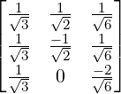 and PT AP =
  . Hence, f(x,y,z) = 0 reduces to
So,
the standard form of the quadric is 4
z12 +
z22 +
z32 =
 ,
, where

=
P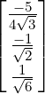
=

is the
center and
x +
y +
z = 0
,x - y = 0 and
x +
y - 2
z = 0 as the principal axes.
Part 2 Here f(x,y,z) = 0 reduces to  -
- -
- = 1 which is the equation of a
hyperboloid consisting of two sheets with center 0 and the axes x, y and z as the principal
axes.
= 1 which is the equation of a
hyperboloid consisting of two sheets with center 0 and the axes x, y and z as the principal
axes.
Part 3 Here f(x,y,z) = 0 reduces to  -
- +
+  = 1 which is the equation of a
hyperboloid consisting of one sheet with center 0 and the axes x, y and z as the principal
axes.
= 1 which is the equation of a
hyperboloid consisting of one sheet with center 0 and the axes x, y and z as the principal
axes.
Part 4 Here f(x,y,z) = 0 reduces to z = y2 - 3x2 + 10 which is the equation of a hyperbolic
paraboloid.
The different curves are given in Figure 6.5. These curves have been drawn using the package
“MATHEMATICA”.

 DRAFT
DRAFT

 DRAFT
DRAFT

 DRAFT
DRAFT


![[ ]
1 1
- 1 - 1](LA1886x.png) . Then,
. Then, ![[ ]
1
1](LA1887x.png) is a left eigenvector of
is a left eigenvector of ![( [ ])
1
0,y = - 1](LA1888x.png) is a (right) eigenpair of
is a (right) eigenpair of 

![[ ]
1 1
2 2](LA1889x.png) . Then,
. Then, ![( [ ])
1
0,x = - 1](LA1890x.png) and
and ![( [ ])
1
3,y = 2](LA1891x.png) are (right) eigen-pairs of
are (right) eigen-pairs of
![( [ ])
3,u = 1
1](LA1892x.png) and
and ![( [ ])
0,v = 2
- 1](LA1893x.png) are left eigen-pairs of
are left eigen-pairs of 


![[ ]
0 0
0 0](LA1914x.png)
![[ ]
0 1
0 0](LA1915x.png)


![P*AP = P* [Av1, ...,Avk,Avk+1, ...,Avn ]
⌊ ⌋ ⌊ | ⌋
v *1 α ⋅⋅⋅ 0 |* ⋅⋅⋅ *
|| ..|| || .. | ||
|| .|| ||0 . 0 |* ⋅⋅⋅ *||
|| v *k|| ||0--⋅⋅⋅--α-|*--⋅⋅⋅-*||
= |v * |[αv1,...,αvk, *,...,*] = |0 ⋅⋅⋅ 0 |* ⋅⋅⋅ *| .
|| k+1.|| || . | ||
|⌈ ..|⌉ |⌈ .. | |⌉
* |
vn 0 ⋅⋅⋅ 0 |* ⋅⋅⋅ *](LA1919x.png)


![⌊ ⌋
α1 0 0
||0 α2 0 ||
AS = [Au1, ...,Aun ] = [α1u1,...,λnun] = [u1,...,un ]|| . . . || = SD,
⌈ .. .. .. ⌉
0 0 α
n](LA1944x.png)

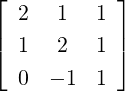 . Then,
 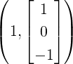 and
and 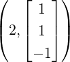 are the only
eigen-pairs. Hence, by Theorem
are the only
eigen-pairs. Hence, by Theorem ![⌊x*⌋
| 1*| [ ]
* * ||x2|| λ1 *
X AX = X [Ax1, Ax2, ...,Axn ] = | ..| [λ1x1,Ax2, ...,Axn ] = 0 B , (6.2.4)
⌈ .⌉
x*n](LA1980x.png)
![[ ] [ ] [ ] [ ] [ ]
( )* 1 0 * 1 0 1 0 λ1 * 1 0
U^ A ^U = * X AX = *
[0 U ][ 0] U [ 0 U ] 0 [ B 0] U
λ1 * 1 0 λ1 * λ1 *
= * = * = .
0 U B 0 U 0 U BU 0 T](LA1984x.png)
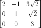


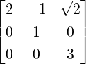
![[ ]
4 4
0 4](LA2004x.png)
![[ ]
10 9
- 4 - 2](LA2005x.png)

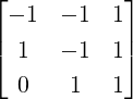
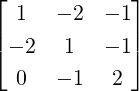


![[ ]
0 B
BT 0](LA2077x.png)
![( [ ])
x
λ, y](LA2078x.png)
![( [ ])
x
- λ, - y](LA2079x.png)
![[ ]
B C
- C B](LA2080x.png)
![[ ]
x
y](LA2081x.png)
![[ - y ]
x](LA2082x.png)
![[ ]
x + iy
- y + ix](LA2083x.png)
![[ x - iy ]
- y - ix](LA2084x.png)
![( [ ])
x + iy
s+ it, - y + ix](LA2087x.png)
![[ ]
2 1
1 2](LA2093x.png) or
or ![[ ]
3 1+ i
1 - i 4](LA2094x.png) . Then,
. Then, ![[ ]
1 1
1 1](LA2095x.png) or
or ![[ √ -- ]
2 1√+-i
1 - i 2](LA2096x.png) . Then,
. Then, ![[ ]
- 2 1
1 - 2](LA2097x.png) or
or ![[ ]
- 2 1- i
1+ i - 2](LA2098x.png) . Then,
. Then, ![[- 1 1 ]
1 - 1](LA2099x.png) or
or ![[ - 2 1- i]
1+ i - 1](LA2100x.png) . Then,
. Then, ![[ ]
0 1
1 - 1](LA2101x.png) or
or ![[ ]
1 1 + i
1 - i 1](LA2102x.png) . Then,
. Then, 


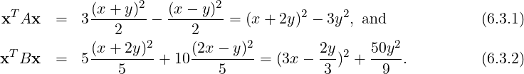


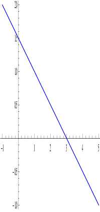
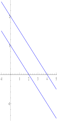
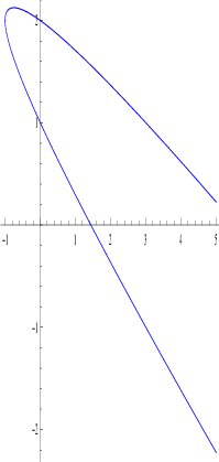


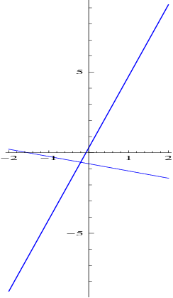
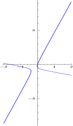
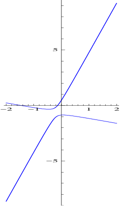
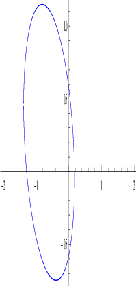


![[ ]
x
y](LA2202x.png) =
= 
![]](LA2204x.png)
![[ ]
u
v](LA2205x.png)